FIULogo_H_CMYKsmaller
Department of Mechanical and Materials Engineering

This is Dr. Levy’s EML3222 System Dynamics Fall 2011 page

Florida International University is a community of faculty, staff and students dedicated to generating and imparting knowledge through 1) excellent teaching and research, 2) the rigorous and respectful exchange of ideas, and 3) community service. All students should respect the right of others to have an equitable opportunity to learn and honestly demonstrate the quality of their learning. Therefore, all students are expected to adhere to a standard of academic conduct, which demonstrates respect for themselves, their fellow students, and the educational mission of the University. All students are deemed by the University to understand that if they are found responsible for academic misconduct, they will be subject to the Academic Misconduct procedures and sanctions, as outlined in the Student Handbook.

Here is the (8/22/2011) updated syllabus for the course.

My office is in EC3474, and email address is levyez@fiu.edu

My tel. no. is 305-348-3643. My fax no. is 305-348-6007/department fax no. is 348-1932

Office hours: T 1-230pm, F 2-330pm

AT PRESENT WE HAVE NO TA. If you need help, please come to see me or write to me.

You will be required to form a group of four students as your study group.

Photocopies of the 3 material selections relating to vibrations will be available in my office starting August 22. Please make up your groups of four and one of you come to my office to get the materials. Cost is $15 per set.

Please start reading the first and second section-Chapter 1 and 2 materials. I will be assigning examples out of those materials starting next week (8/29). So it would be to your benefit to come pick up the copies for your group.

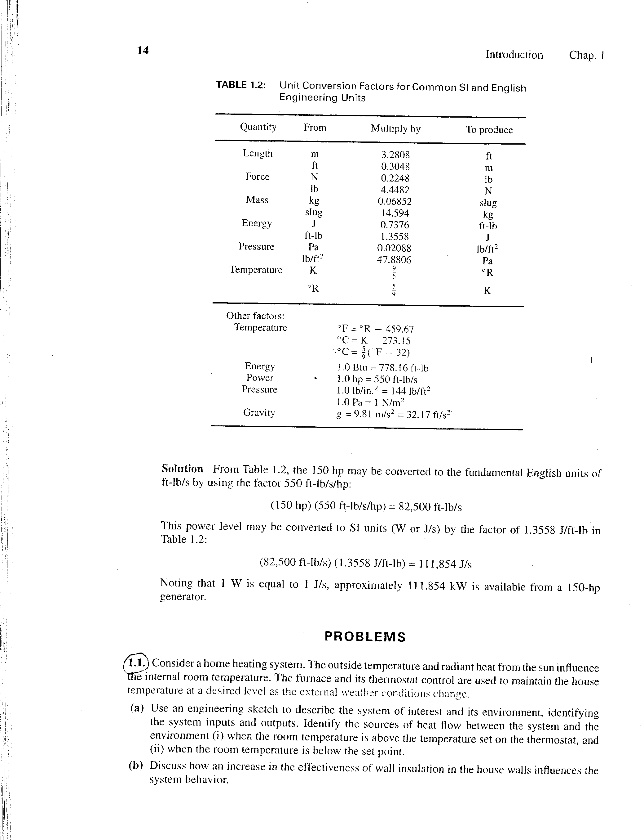
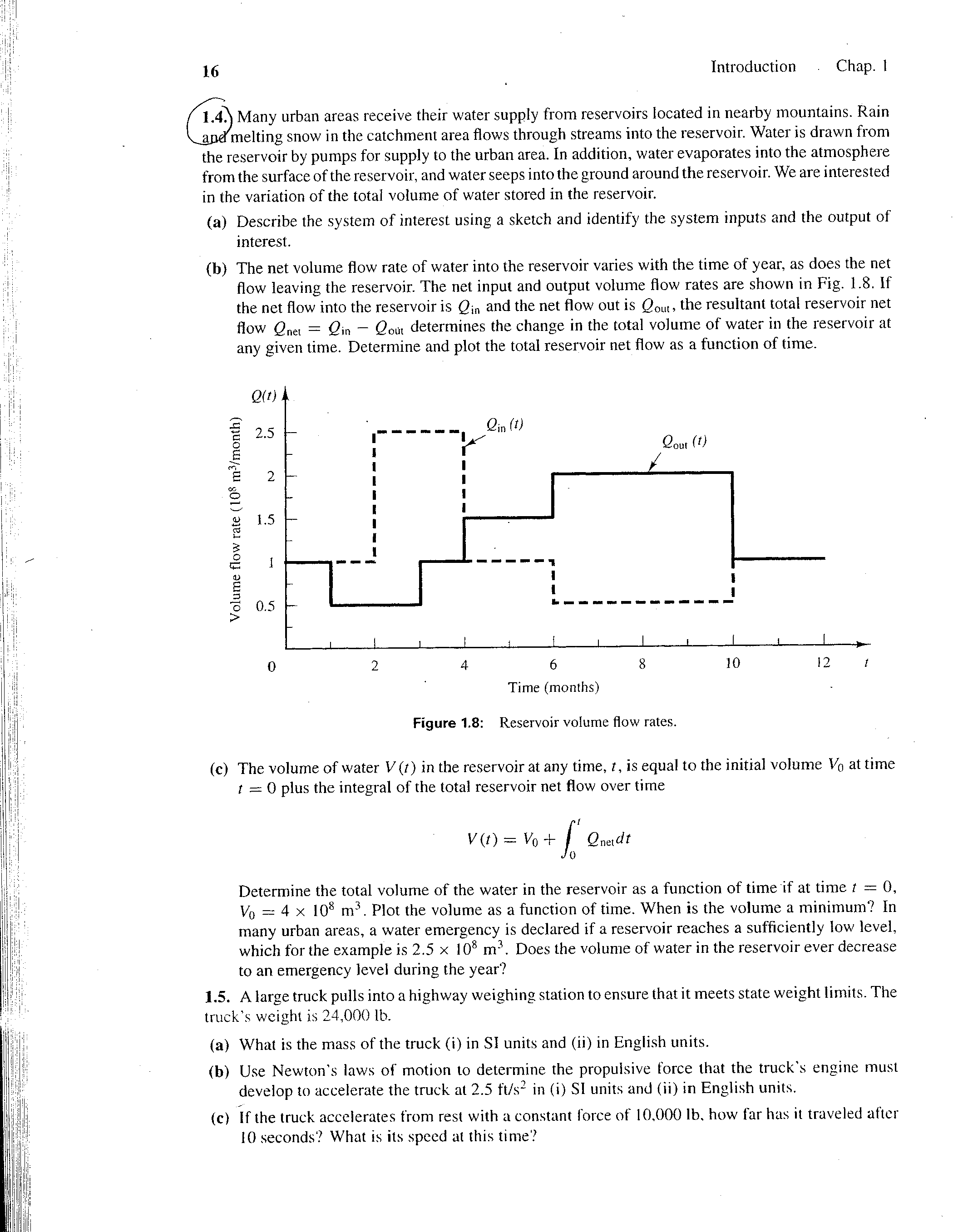
Out of the photocopies of the first two selections do the following: Problems 1.7 to 1.10, 1.13, 1.16, 1.19, 1.22, 1.26, 1.27, 1.29, 1.31, 1.32, and 1.36.

This material and all the linked materials provided, except where stated specifically, are copyrighted © Cesar Levy 2011 and is provided to the students of this course only. Use by any other individual without written consent of the author is forbidden.

PLEASE USE THE WINDOWS MEDIA PLAYER TO VIEW THESE VIDEOS.

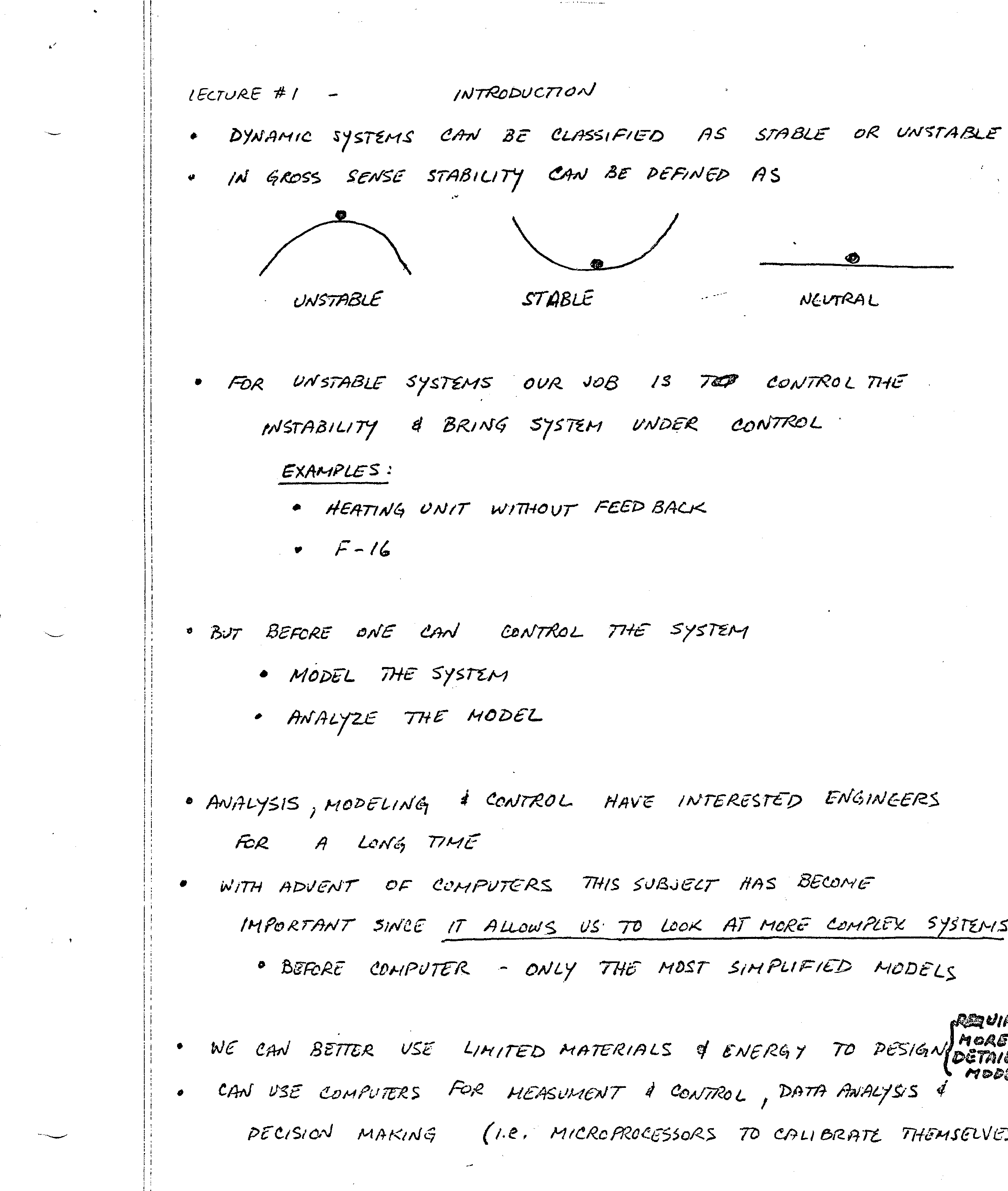
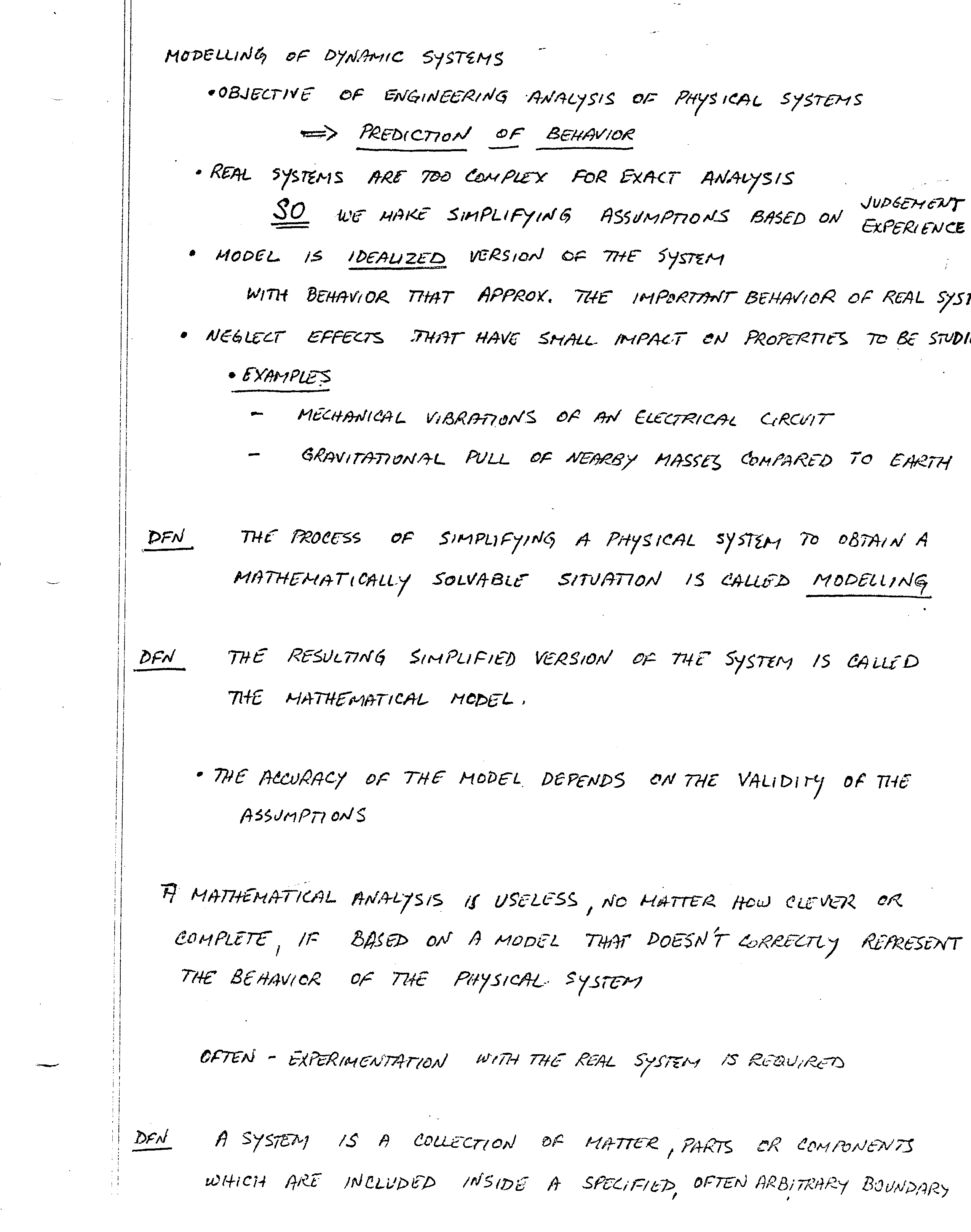
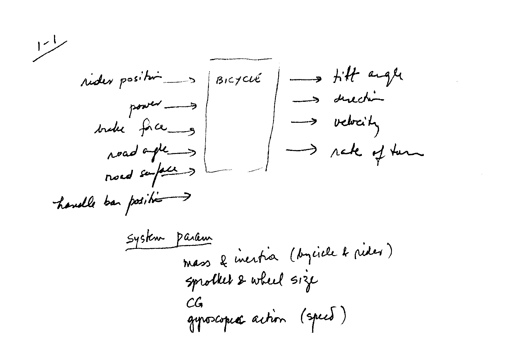
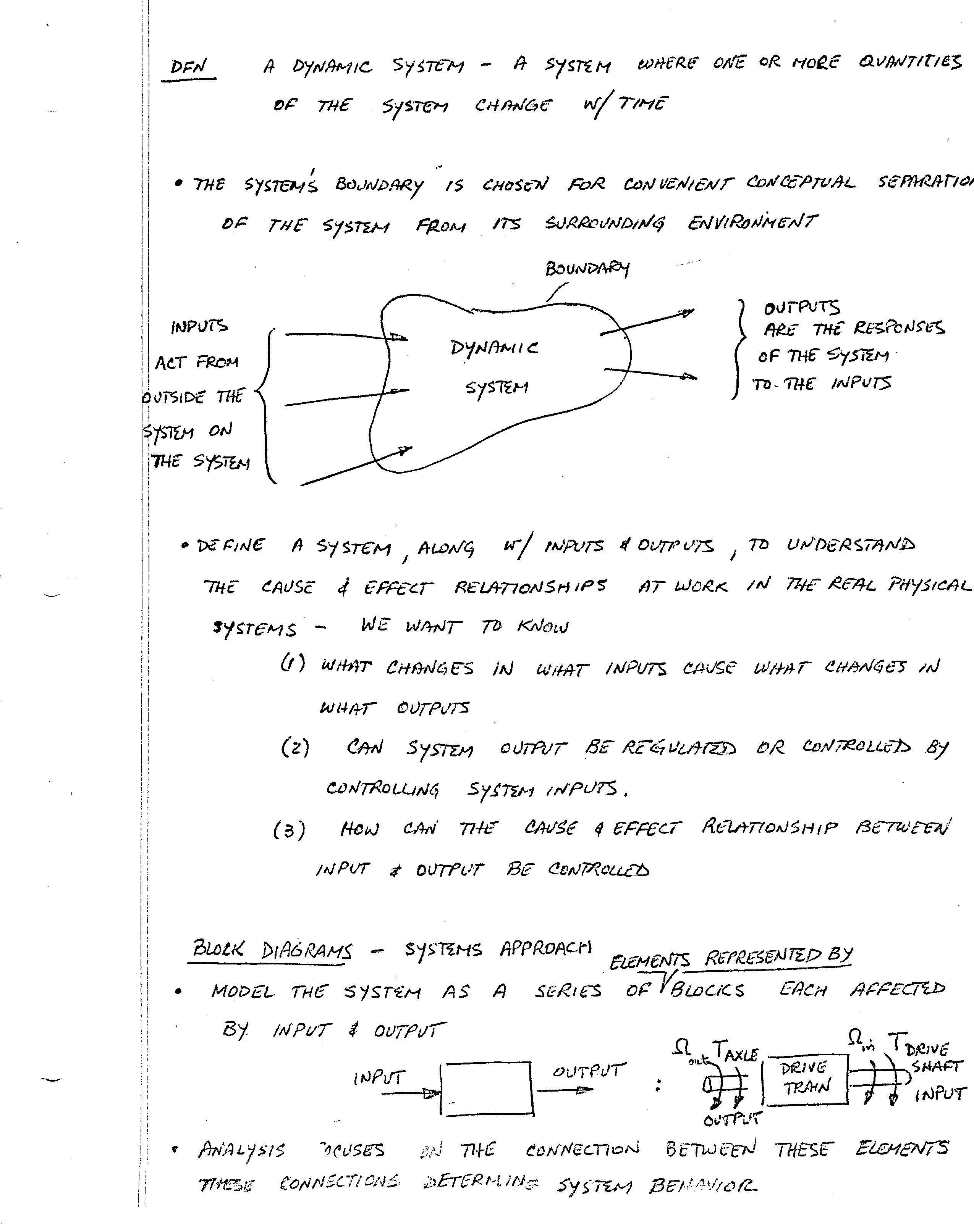
Here is Lecture 1 related video and here are the pages related to that video lecture: page 1, page2, example, page 3, page 4, page 5

Here is Lecture 2 related video and the pages related to the video: page 6, page 7, and page 8

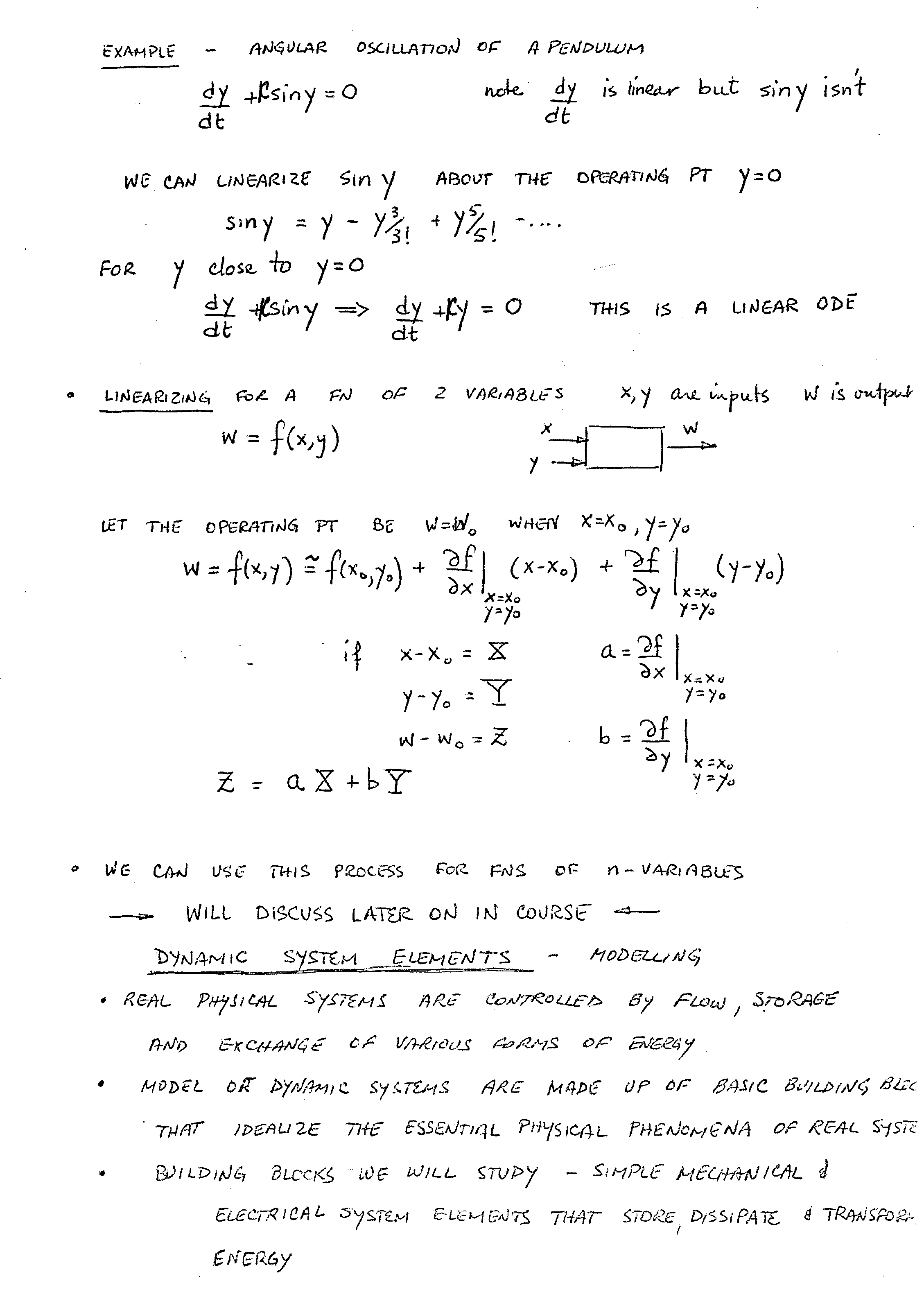
Please make sure that you have the following information about second order systems, namely:

where g is the acceleration of gravity and D_stis the static displacement of the system; that is, weight of the system = k*D_st.

And for systems with damping included: =2ςω_n and =ς and Ccrit=2mω_n =2√mk

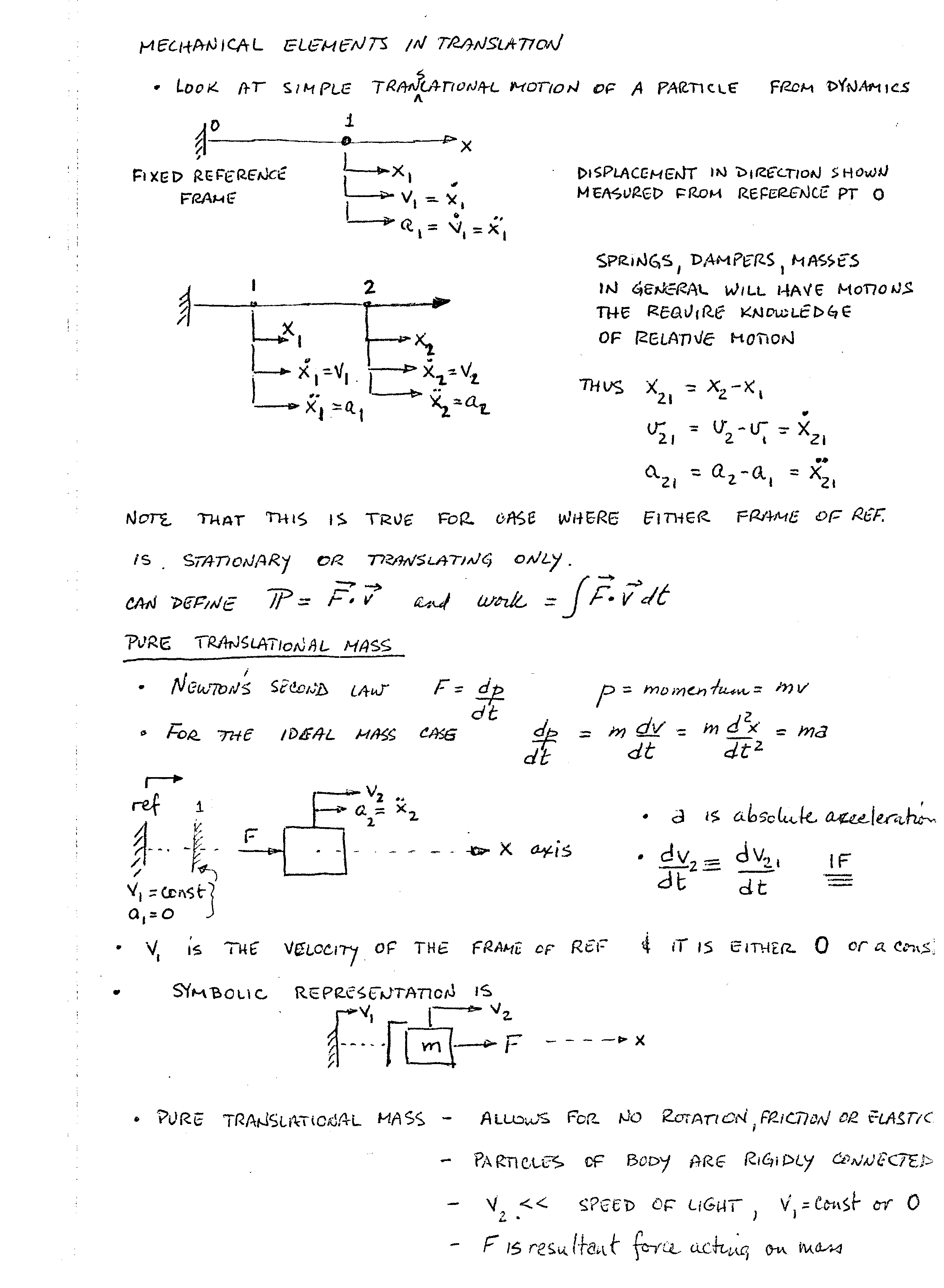
Here is Lecture 3 related video: equation of motion for linear mechanical, linear rotational, inverted pendulum

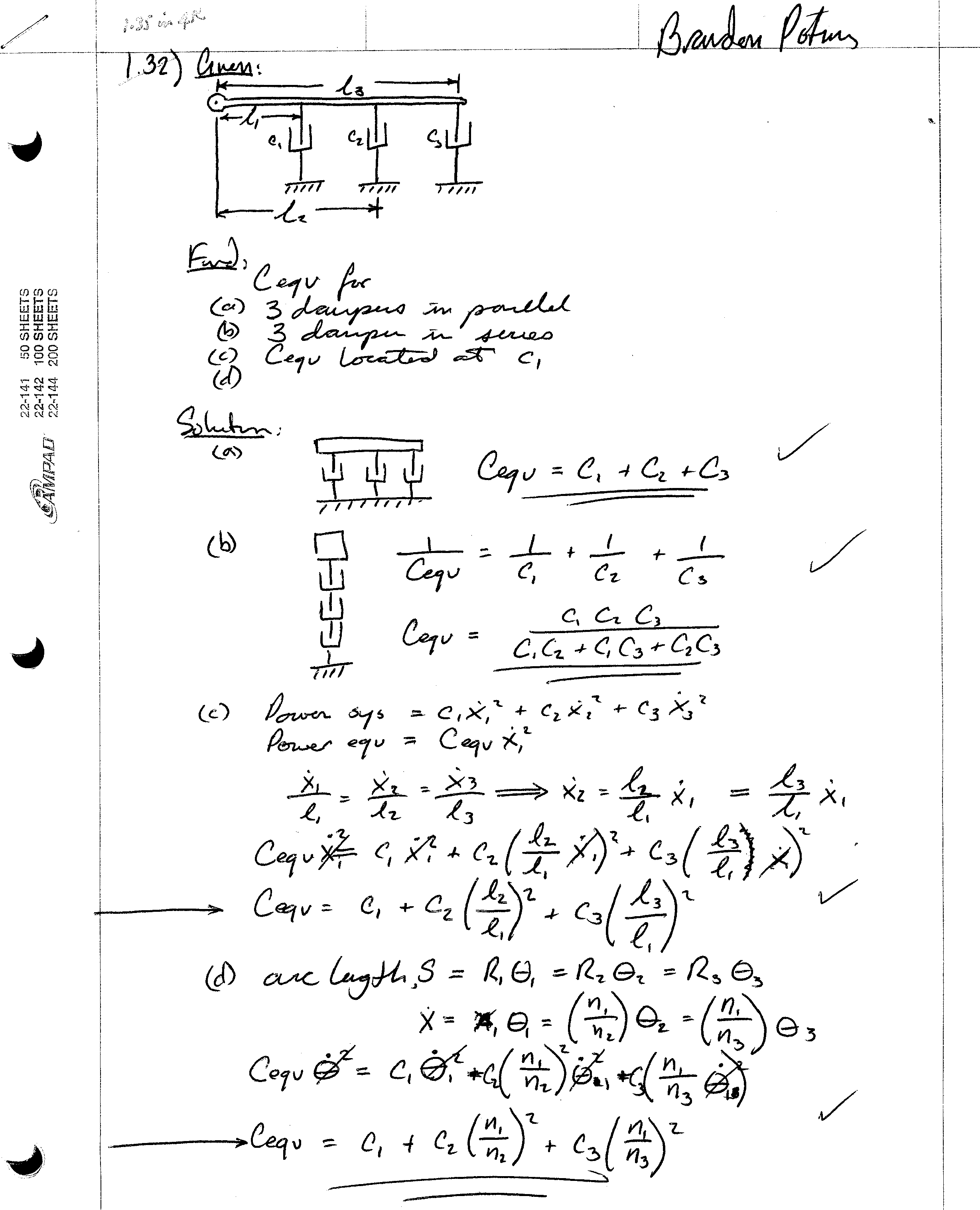
Here is Lecture 4 related video: equivalent springs both linear and rotational, springs in parallel and series

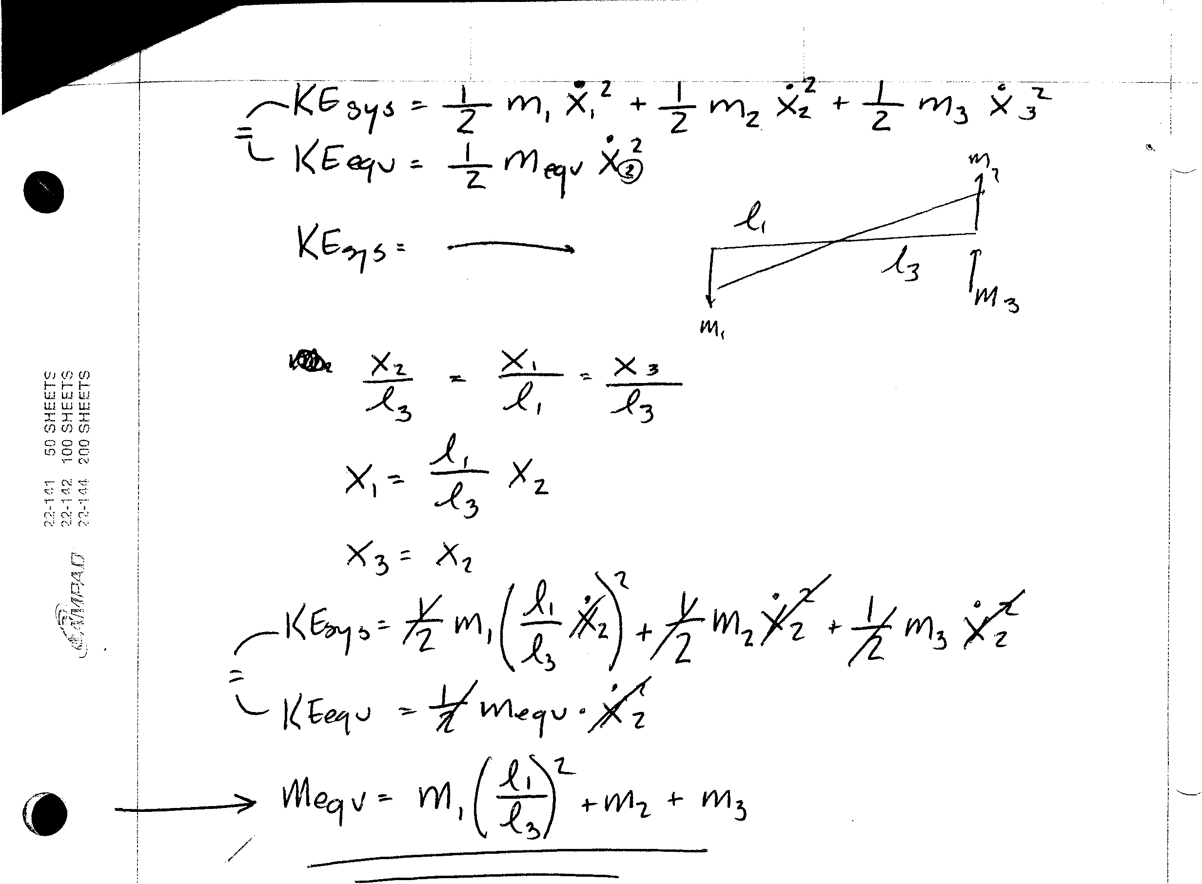
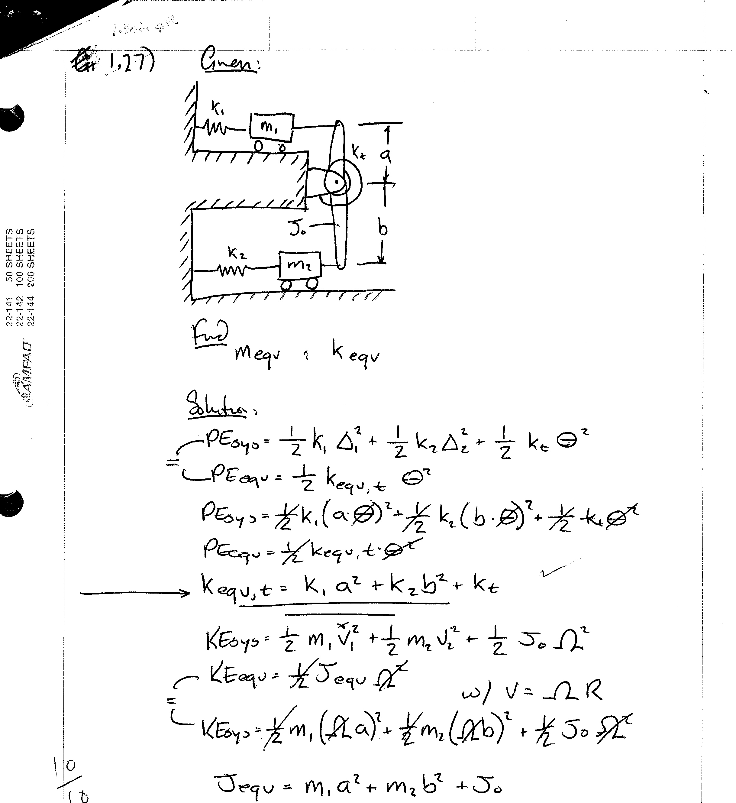
Here is Lecture 5 related video: equivalent springs and masses using equivalent potential and kinetic energies

Here is Lecture 6 related video: we look at damped systems, derive equations and talk about overdamped, critically damped and underdamped systems

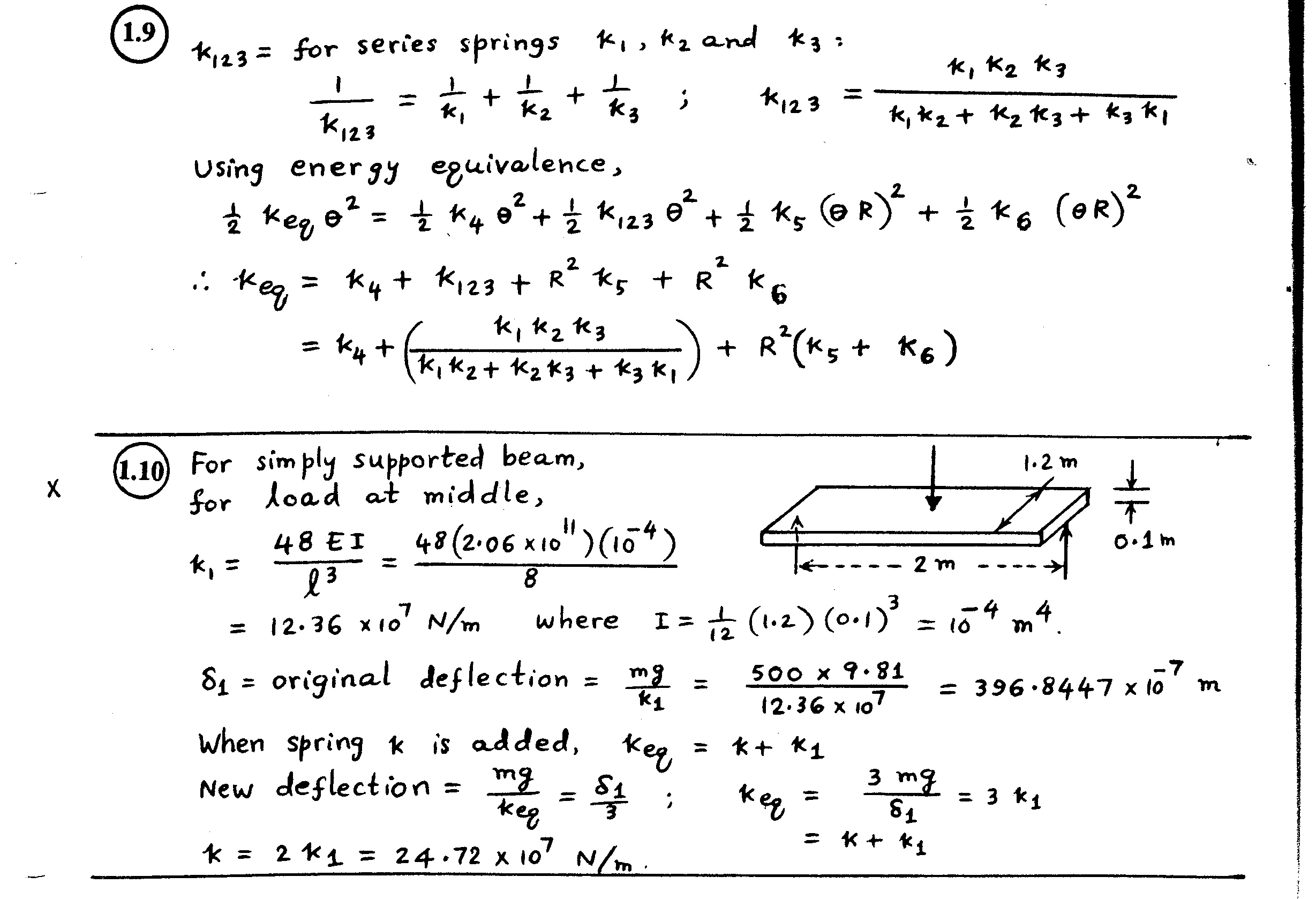
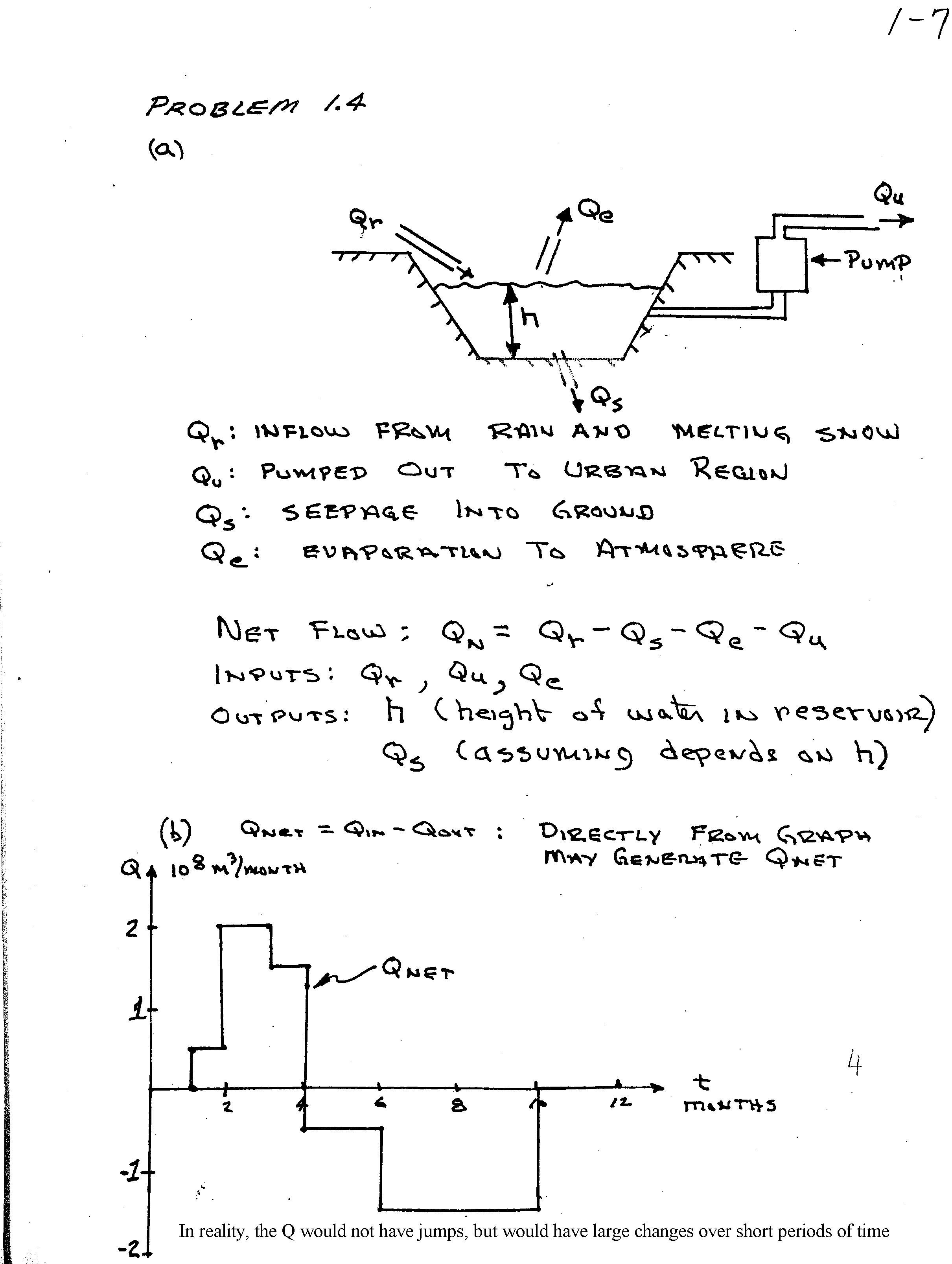
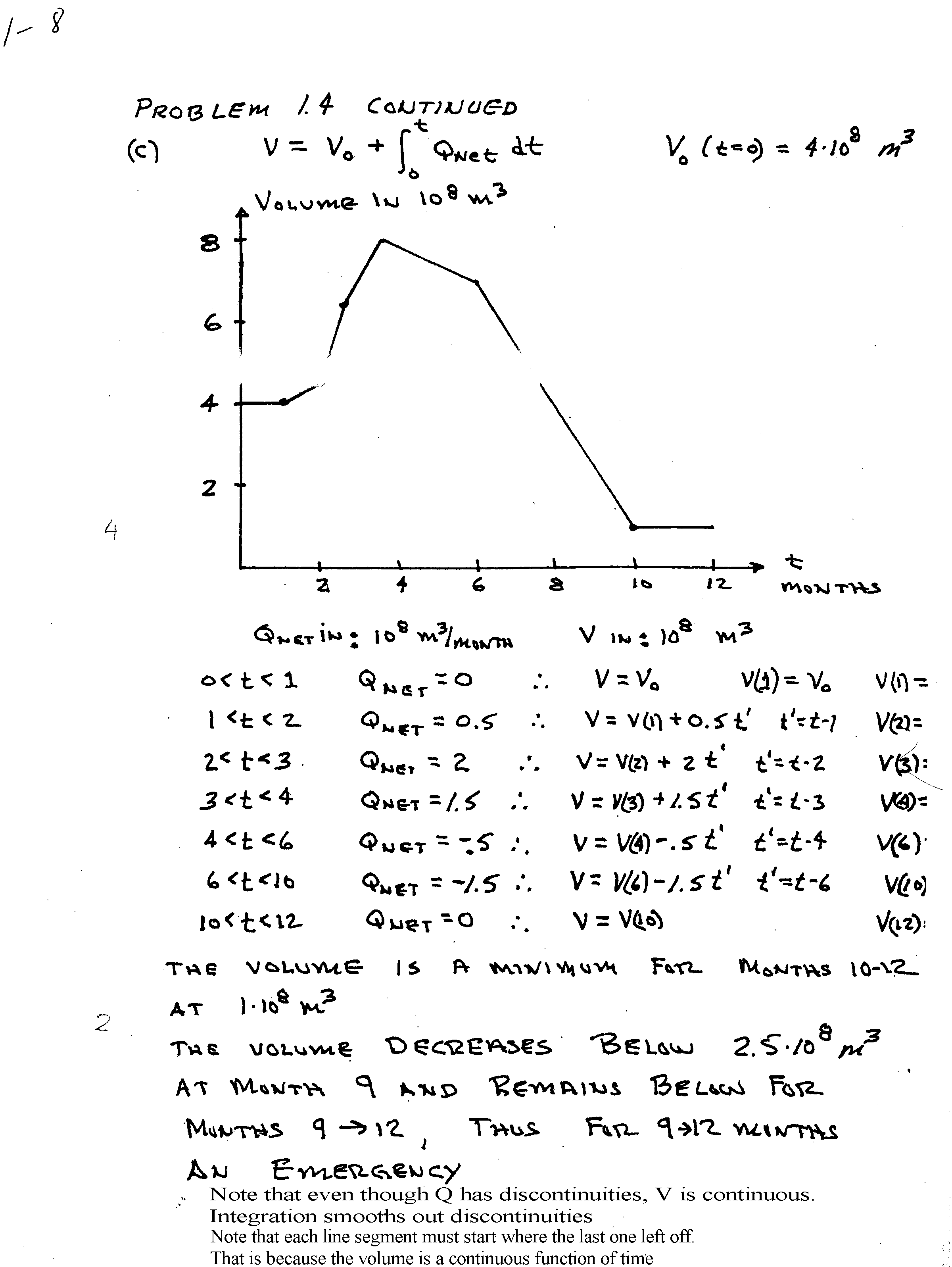
Here are solutions to some of the problems… problems 1-7 and 1-8, 1-9 and 1-10

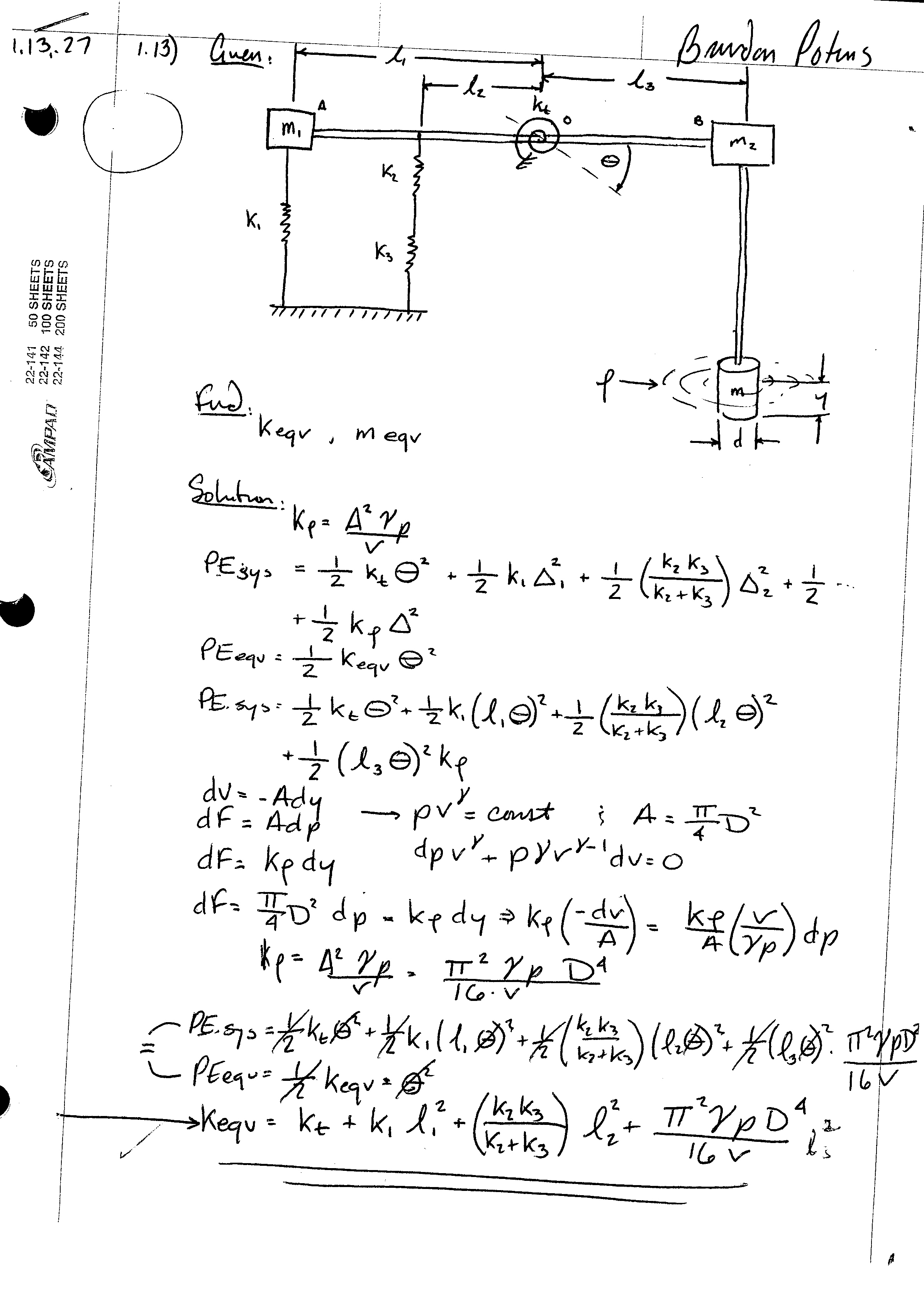
Here are problems 1-13a and 1-13b, 1-29, 1-30, 1-35 and 1-35b

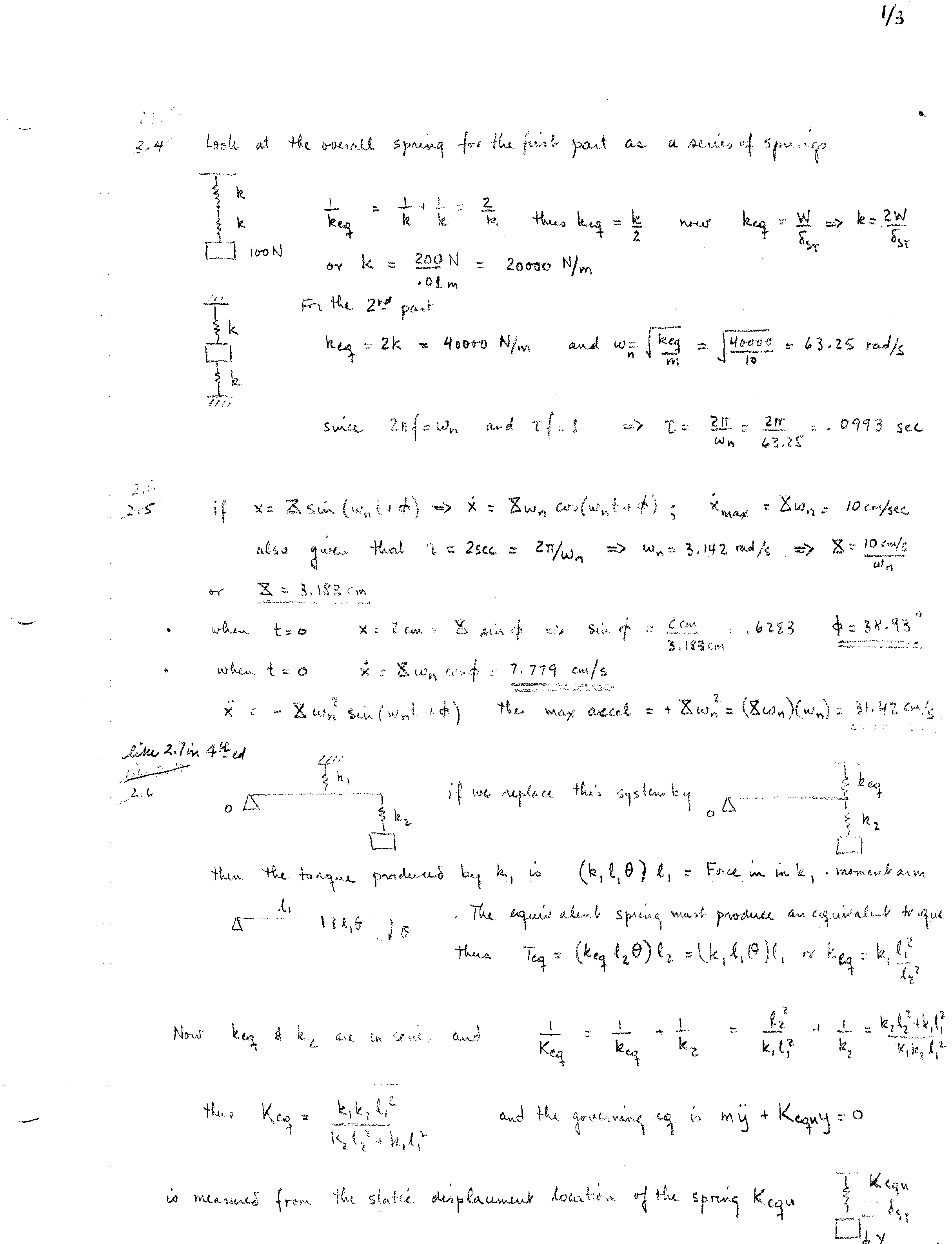
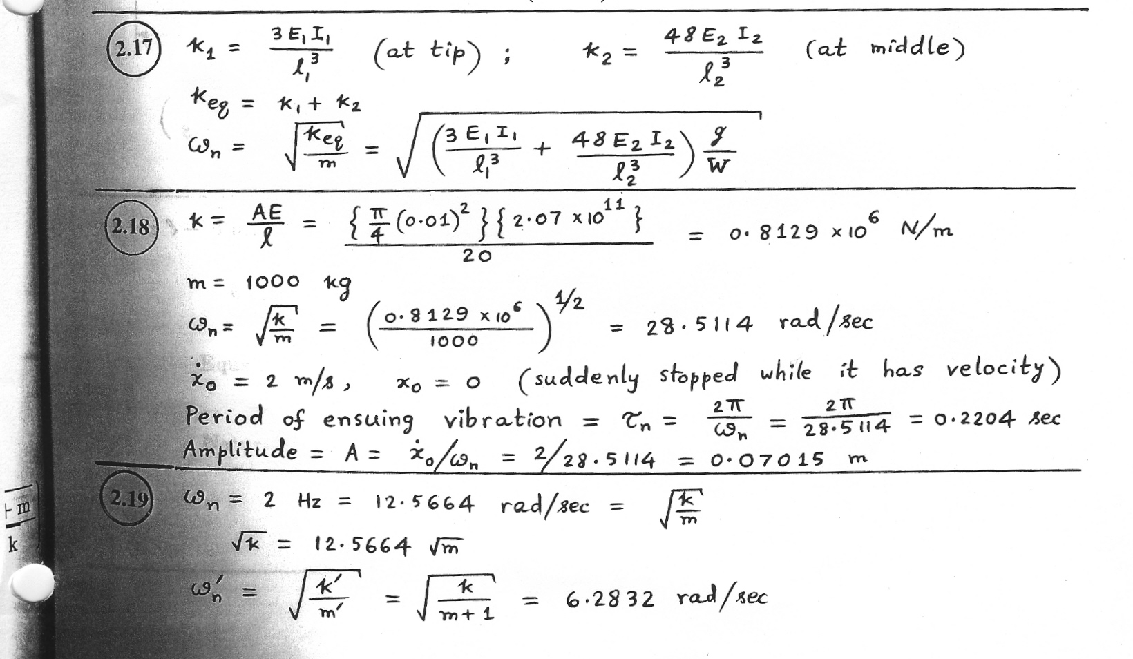
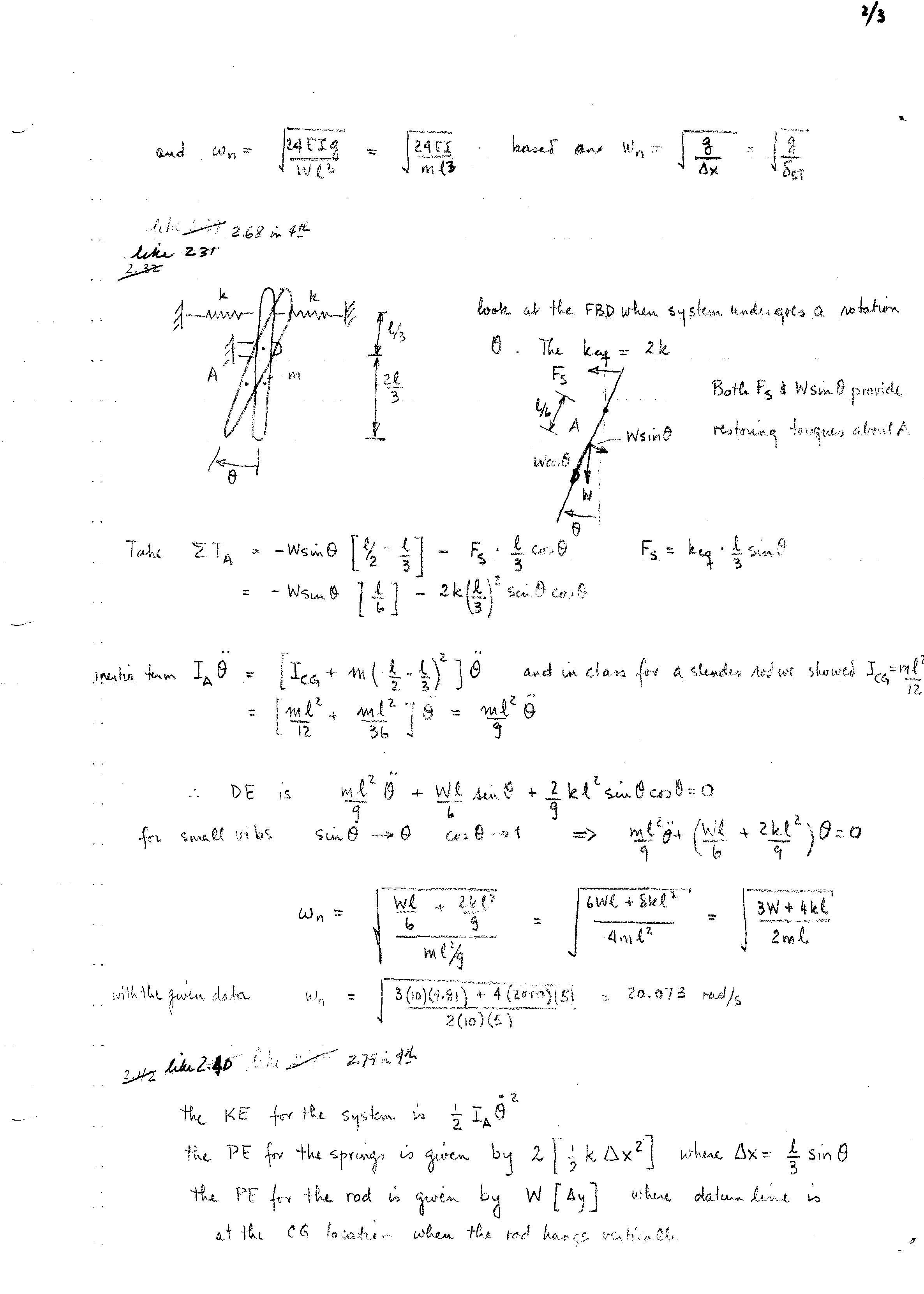
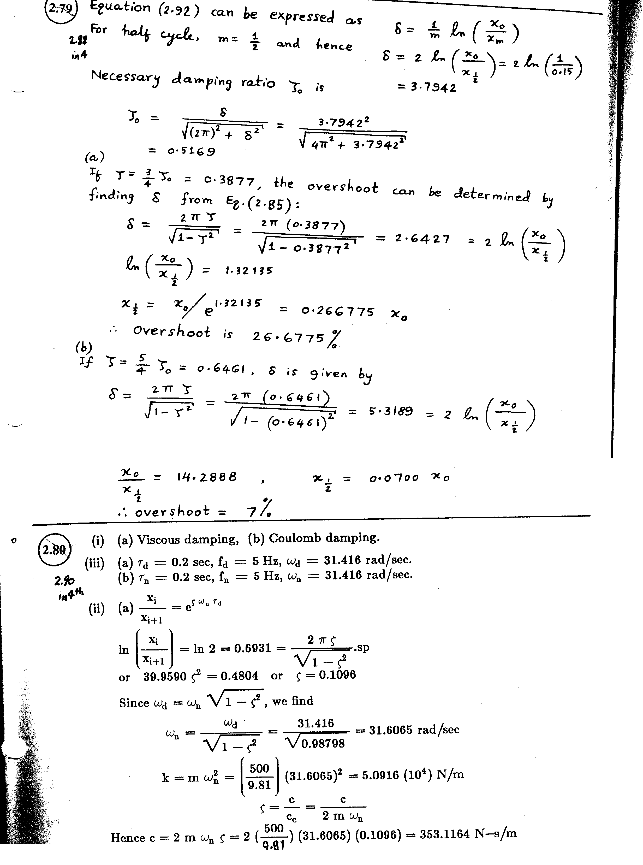
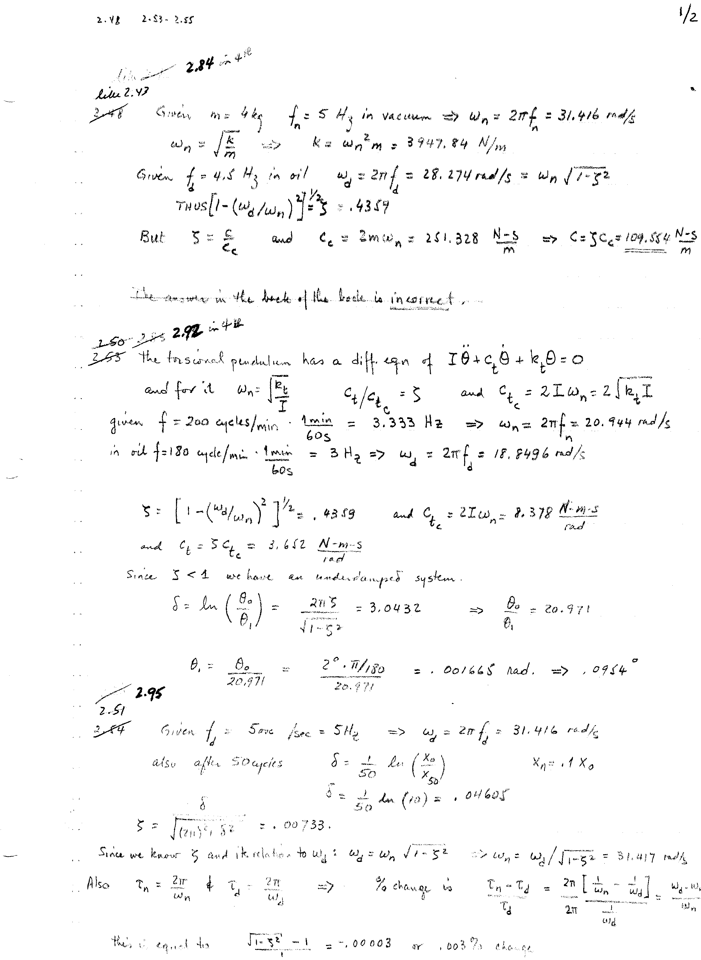
Here is Lecture 7 video: we look at underdamped systems, derived logarithmic decrement and talk about two problems. Look at Problems 2.1-2.4, 2.6, 2.7, 2.17 to 2.19, 2.28, 2.38, 2.45, 2.52, 2.60, 2.80, 2.82, 2.83, and 2.97.

Now for underdamped systems: the logarithmic decrement, δ, equals where ζ is the damping ratio.

Also we showed that δ = (1/N) * ln(x_o/x_N) = (1/N) * ln(x_i/x_i+N)

where N = the number of cycles between the first and last measurement. x here is the displacement and the subscript “o” means the first measurement value. The formula also applies between any N cycles, meaning starting from cycle i and going to cycle i+N.

We will discuss the forced vibration of systems and cover the topic of resonance.

Please start reading Chapters 1 and 2 in the book by Rowell and Wormley.

Here is Lecture 8 video: we look at forced vibration and derive the displacement function for a harmonic force F(t)=P sinw_ft. We discussed the effect of frequency ratio r=w_f/w_n and damping ratio ζ.

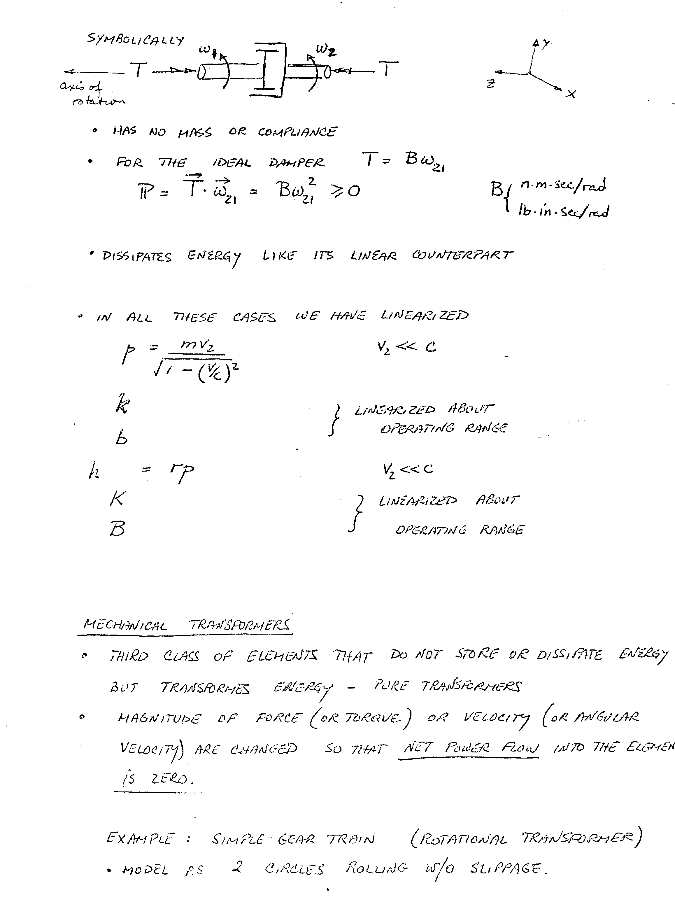
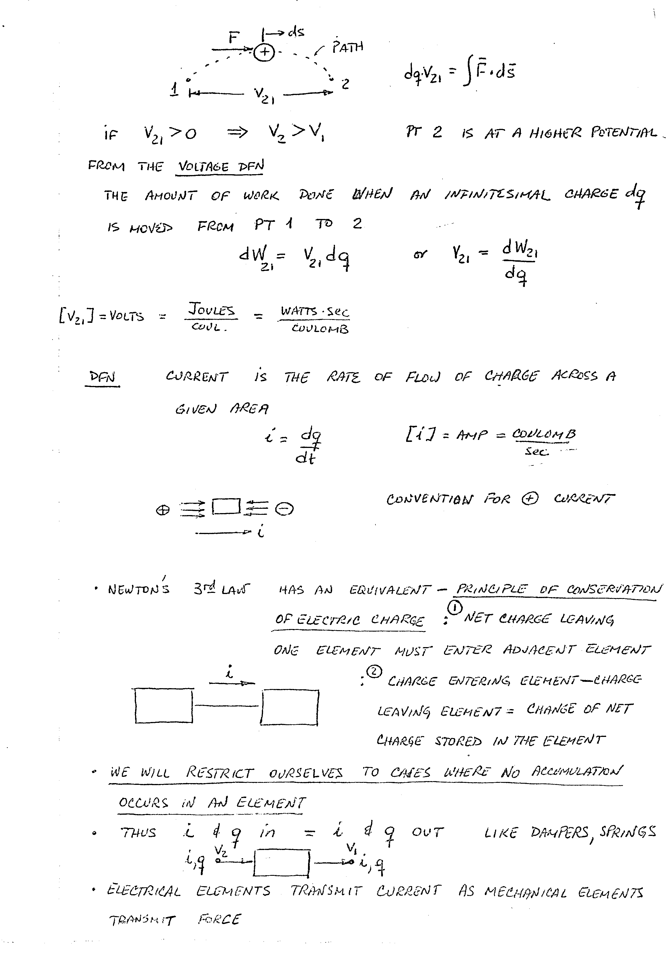
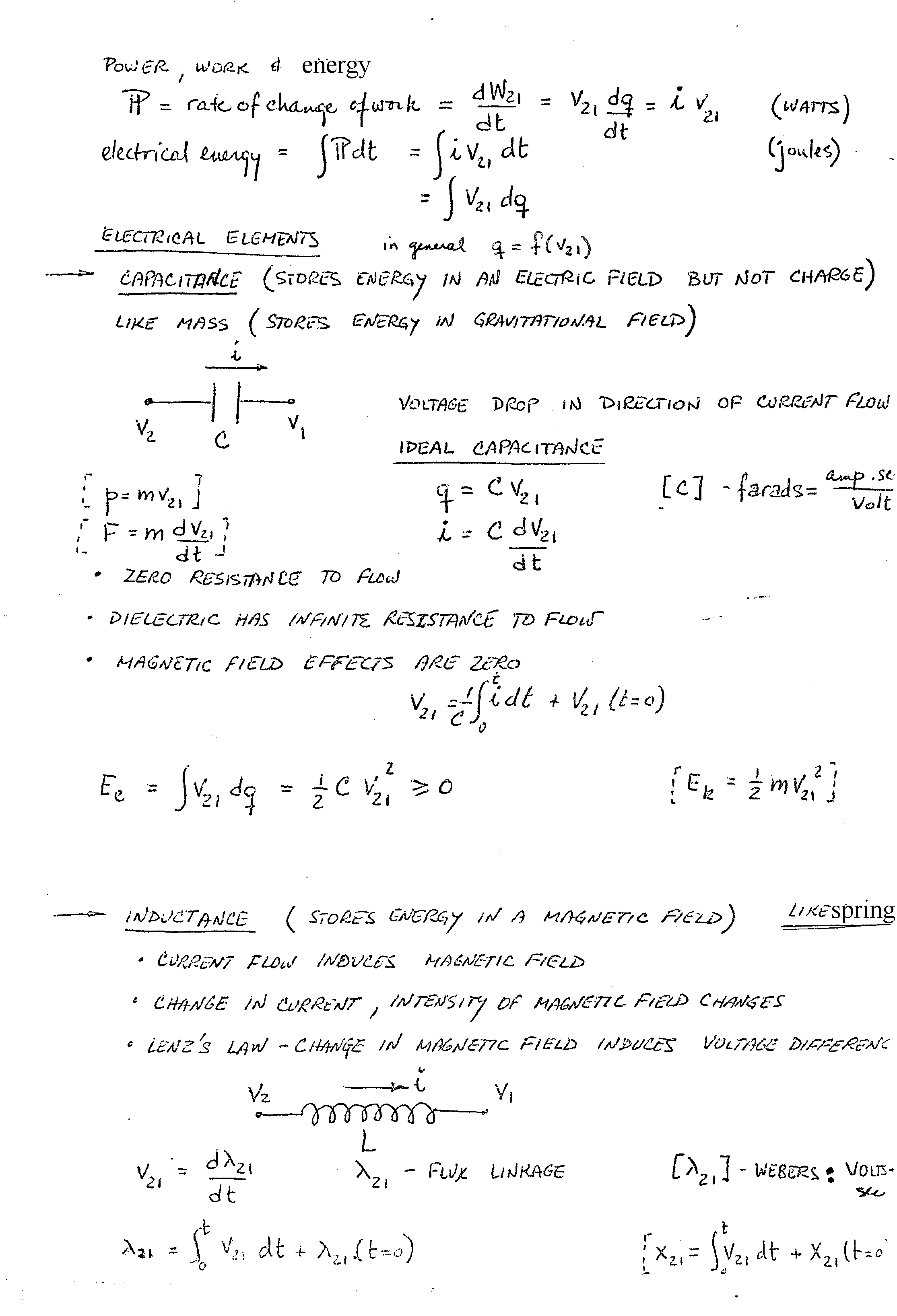
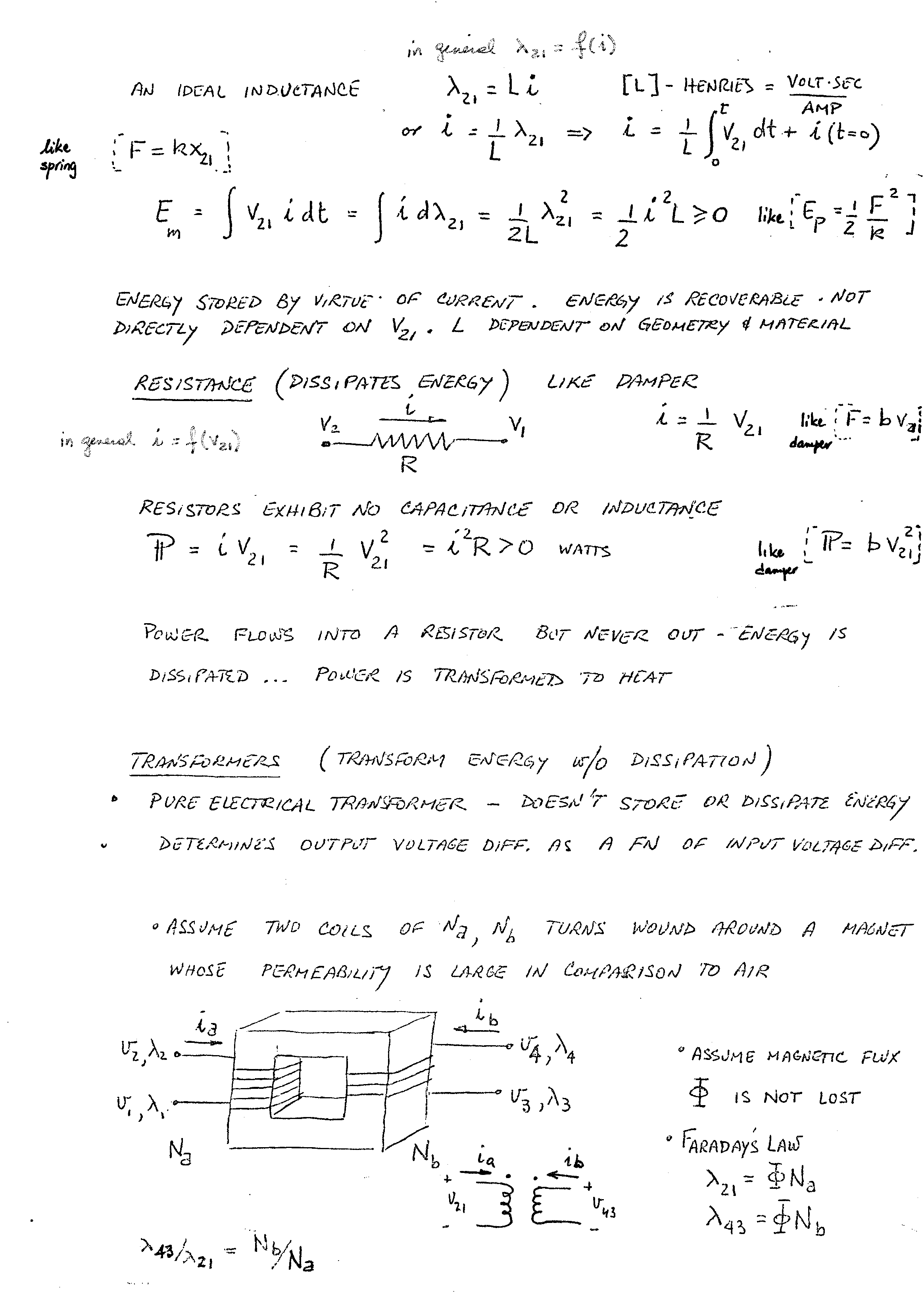
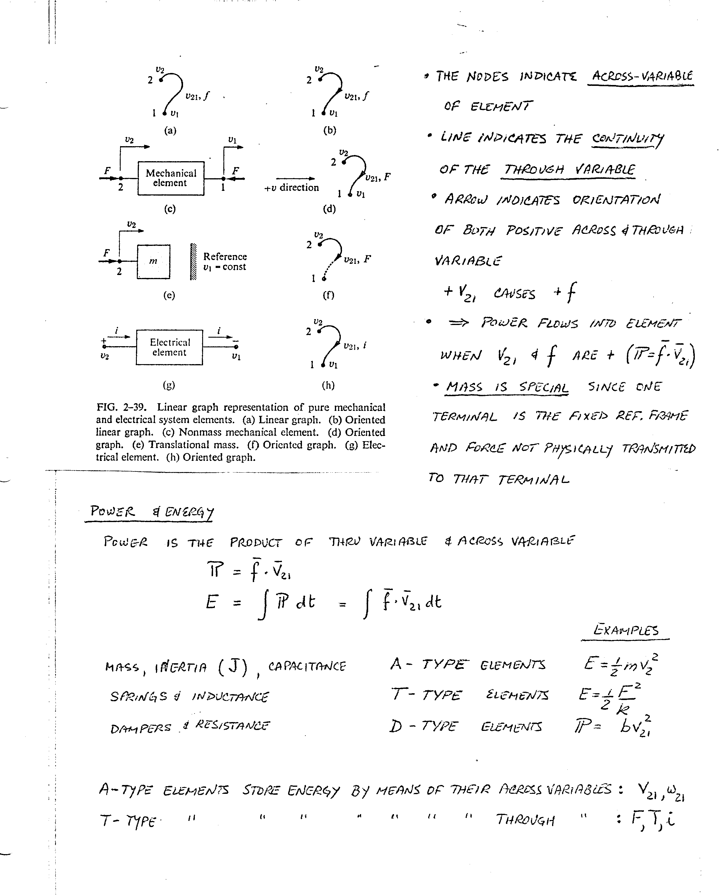
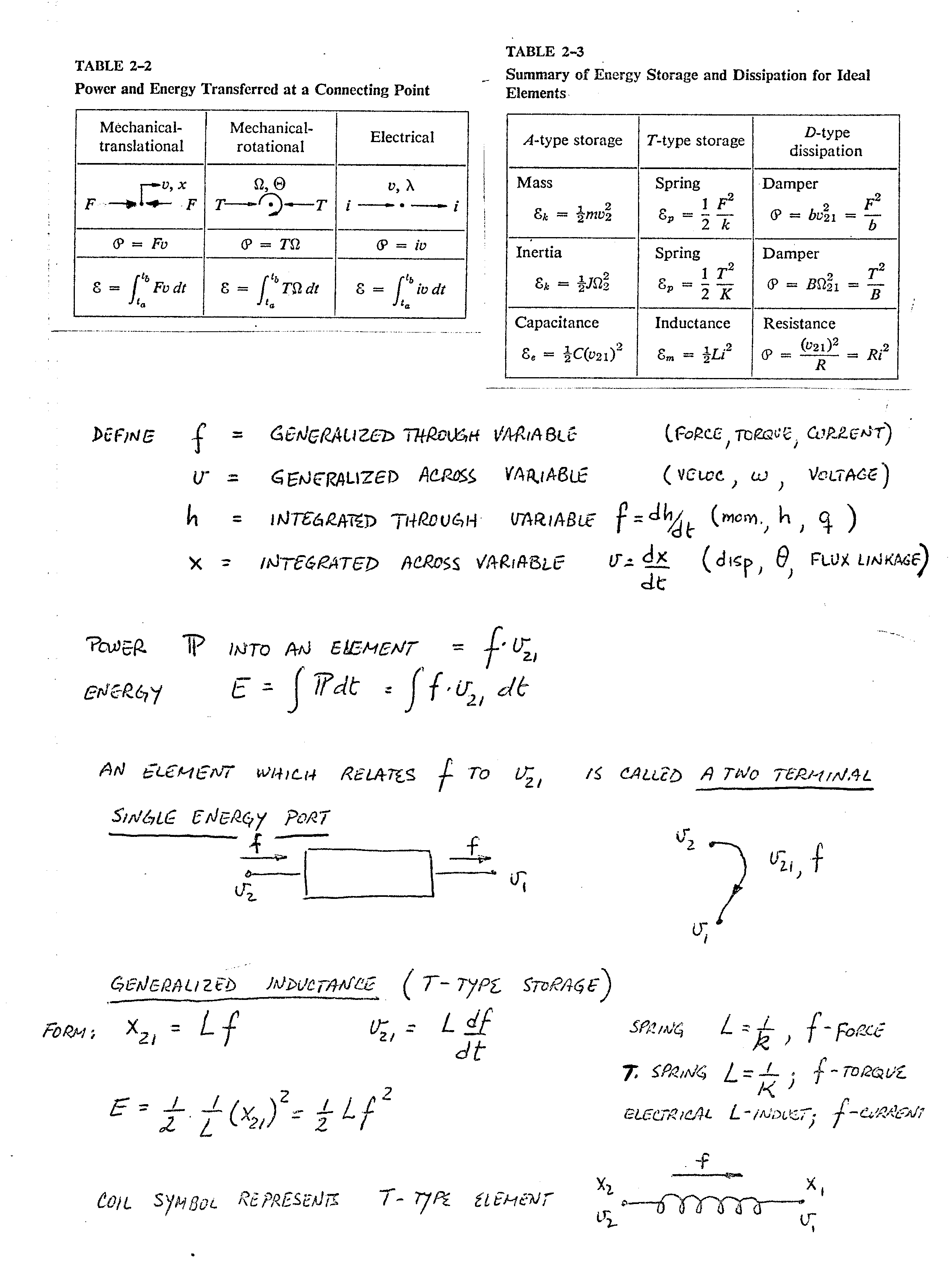
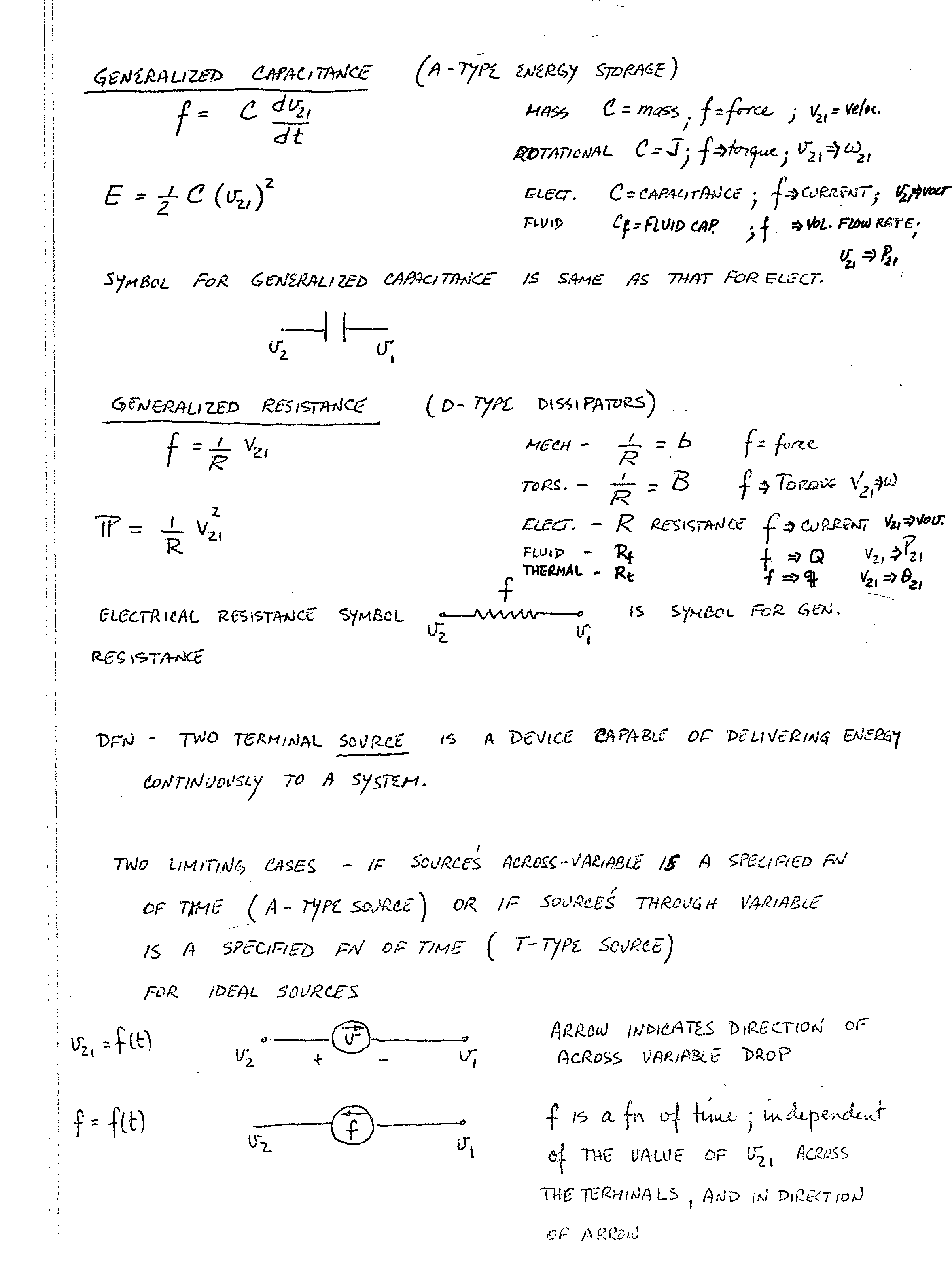
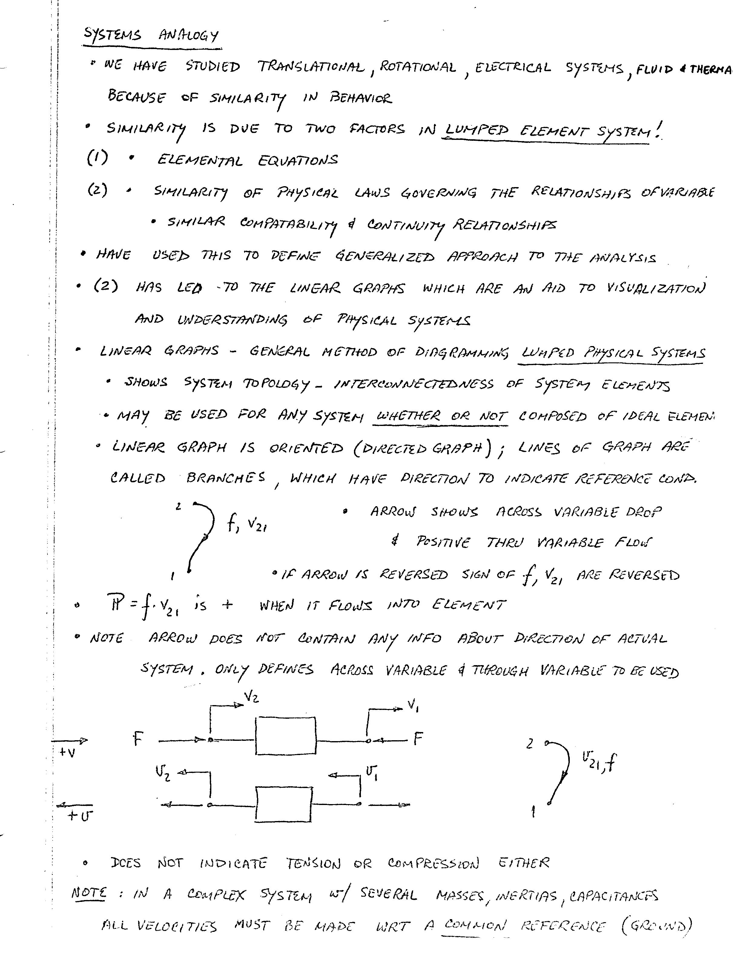
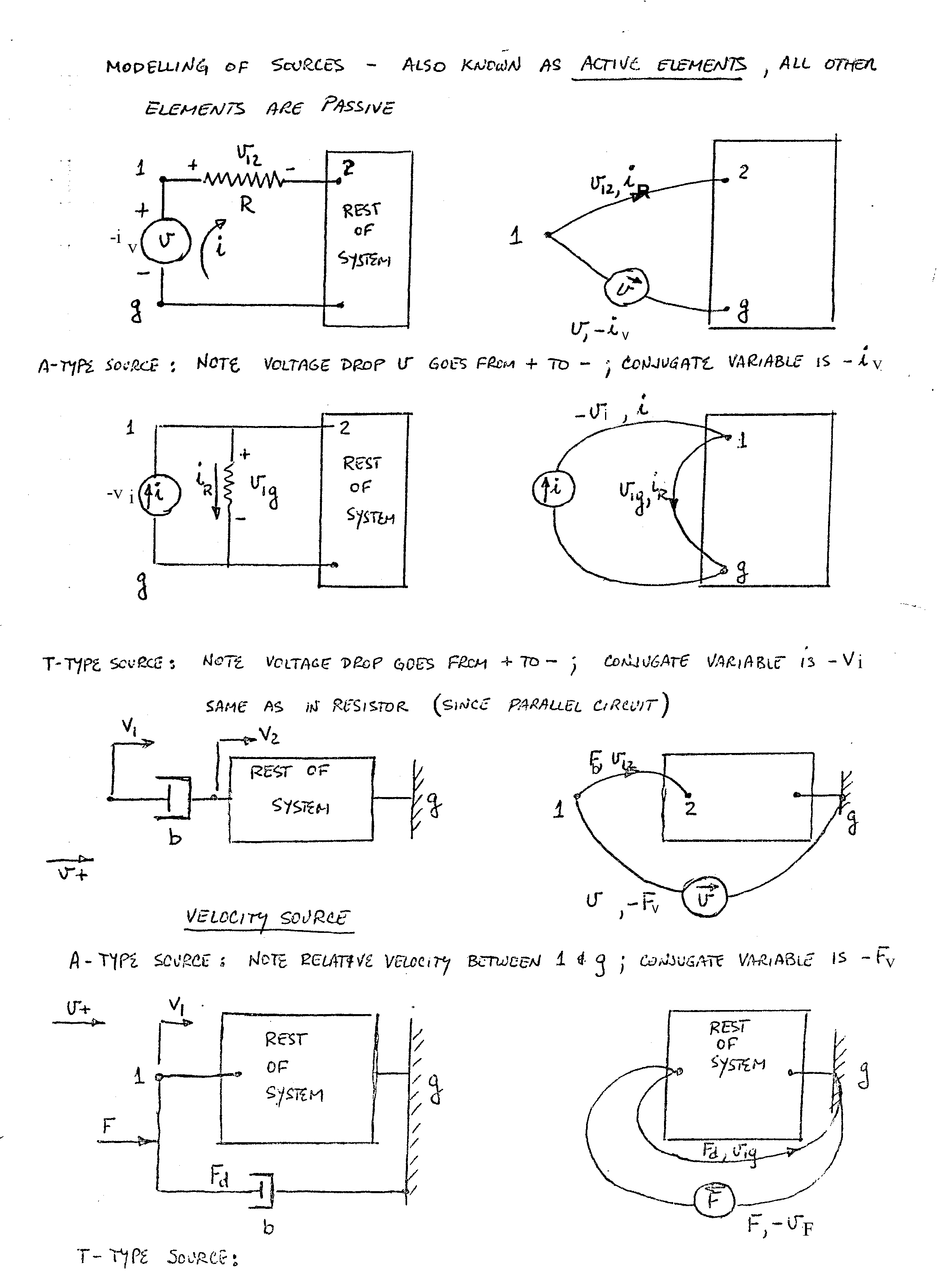
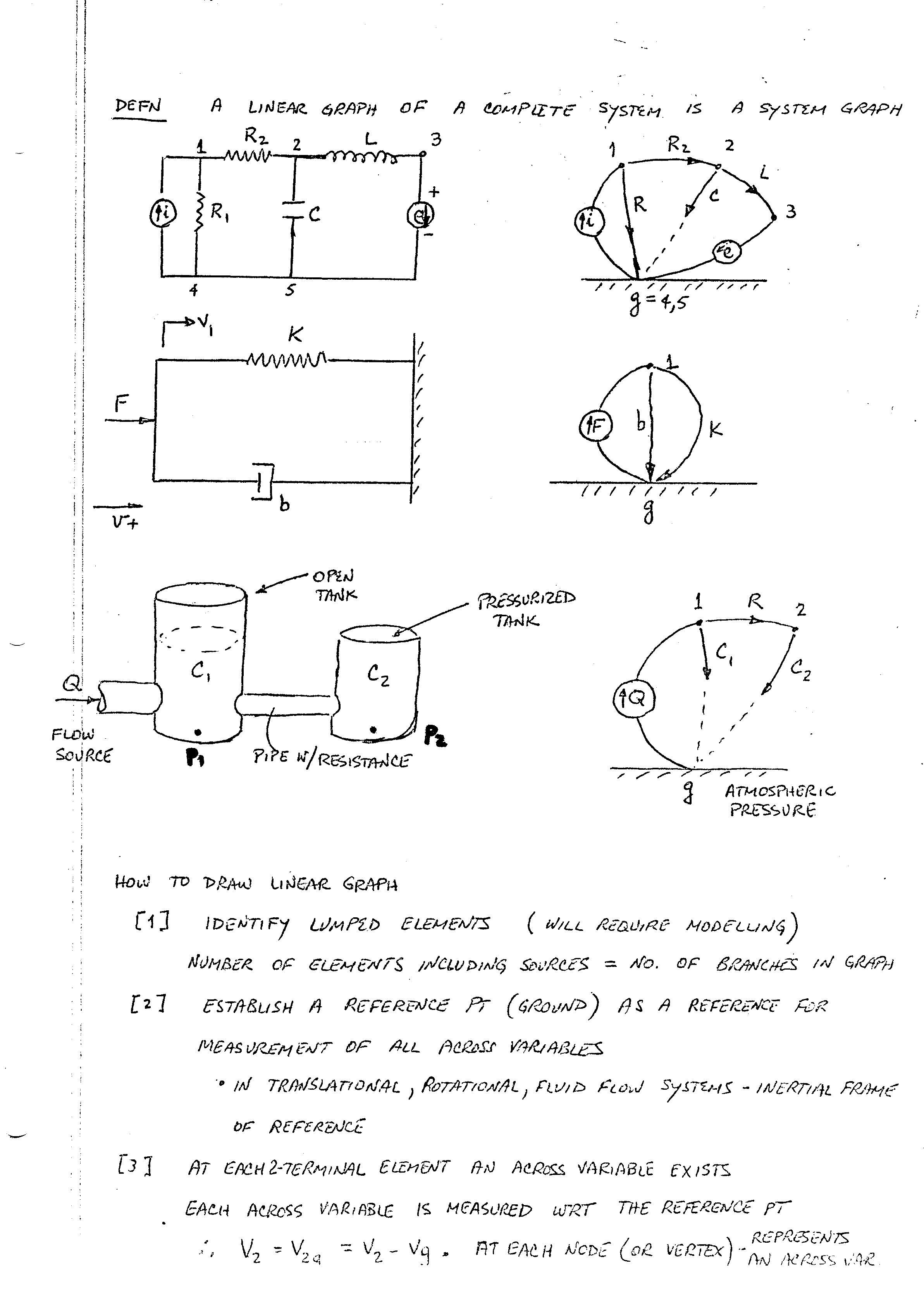
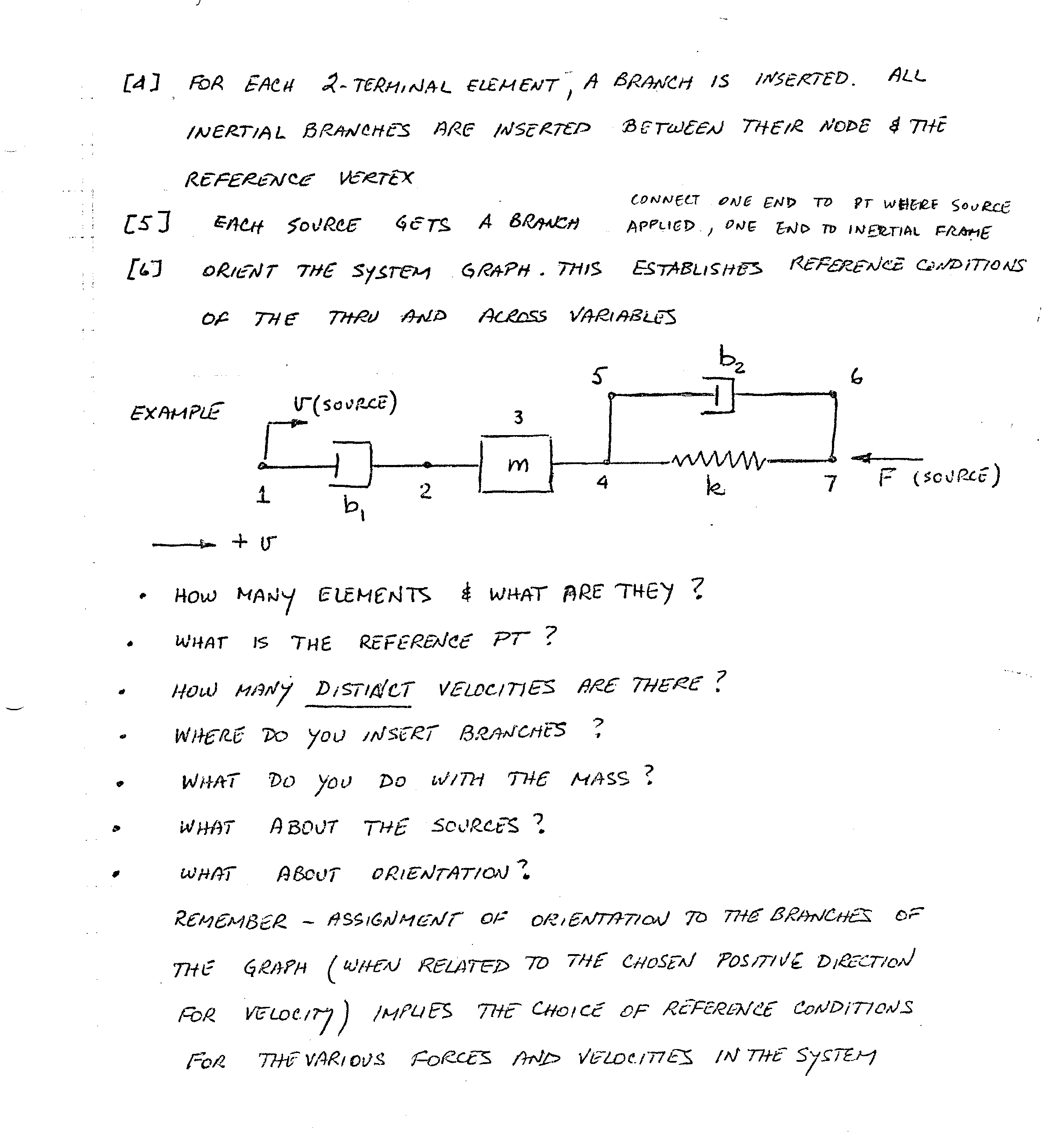
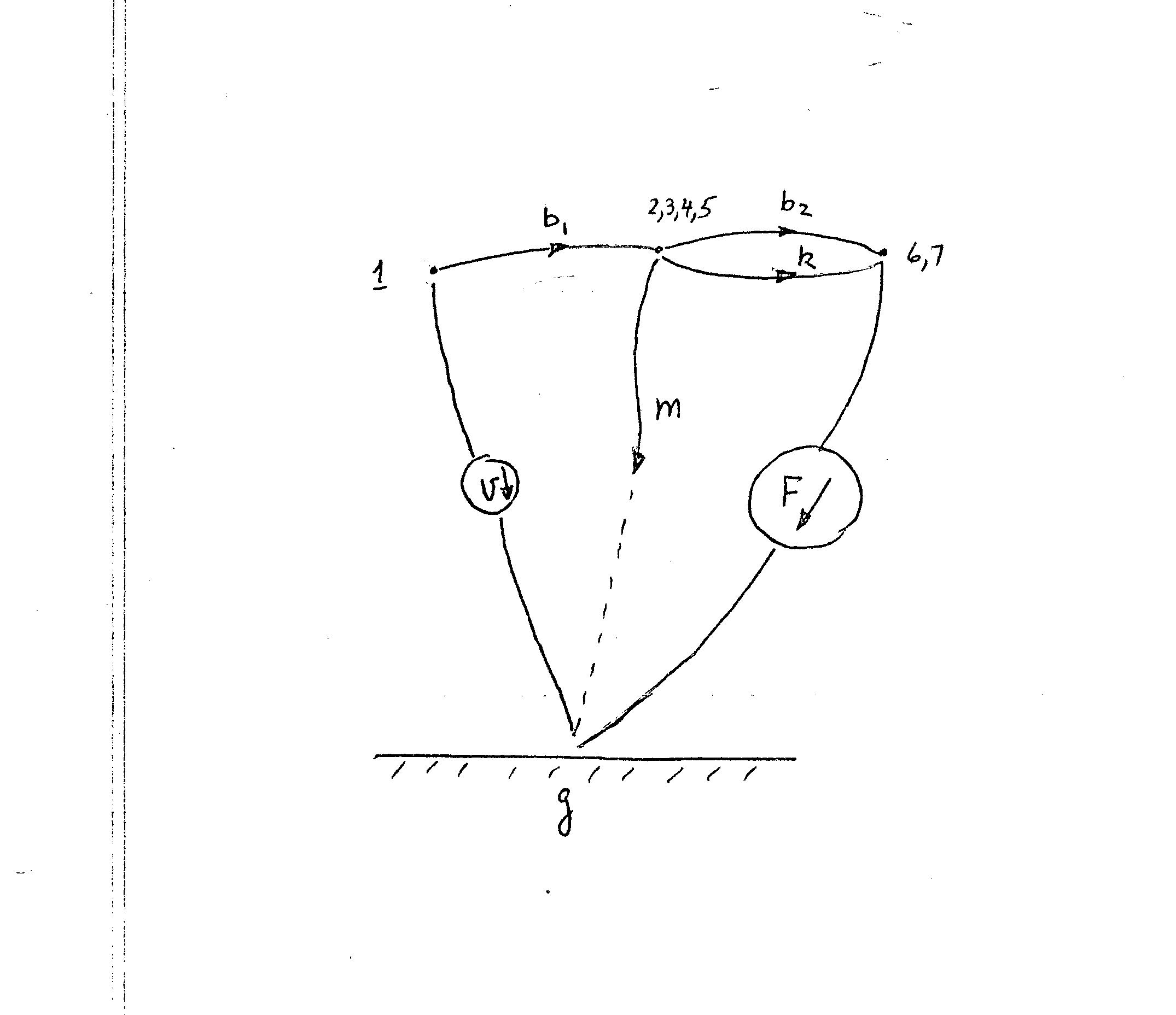
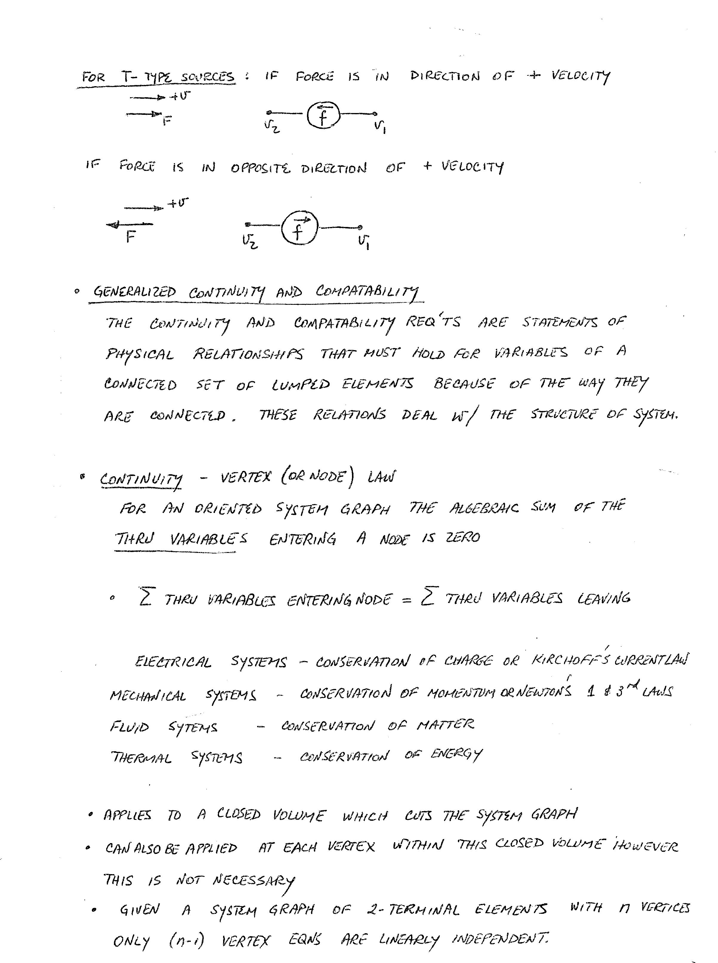
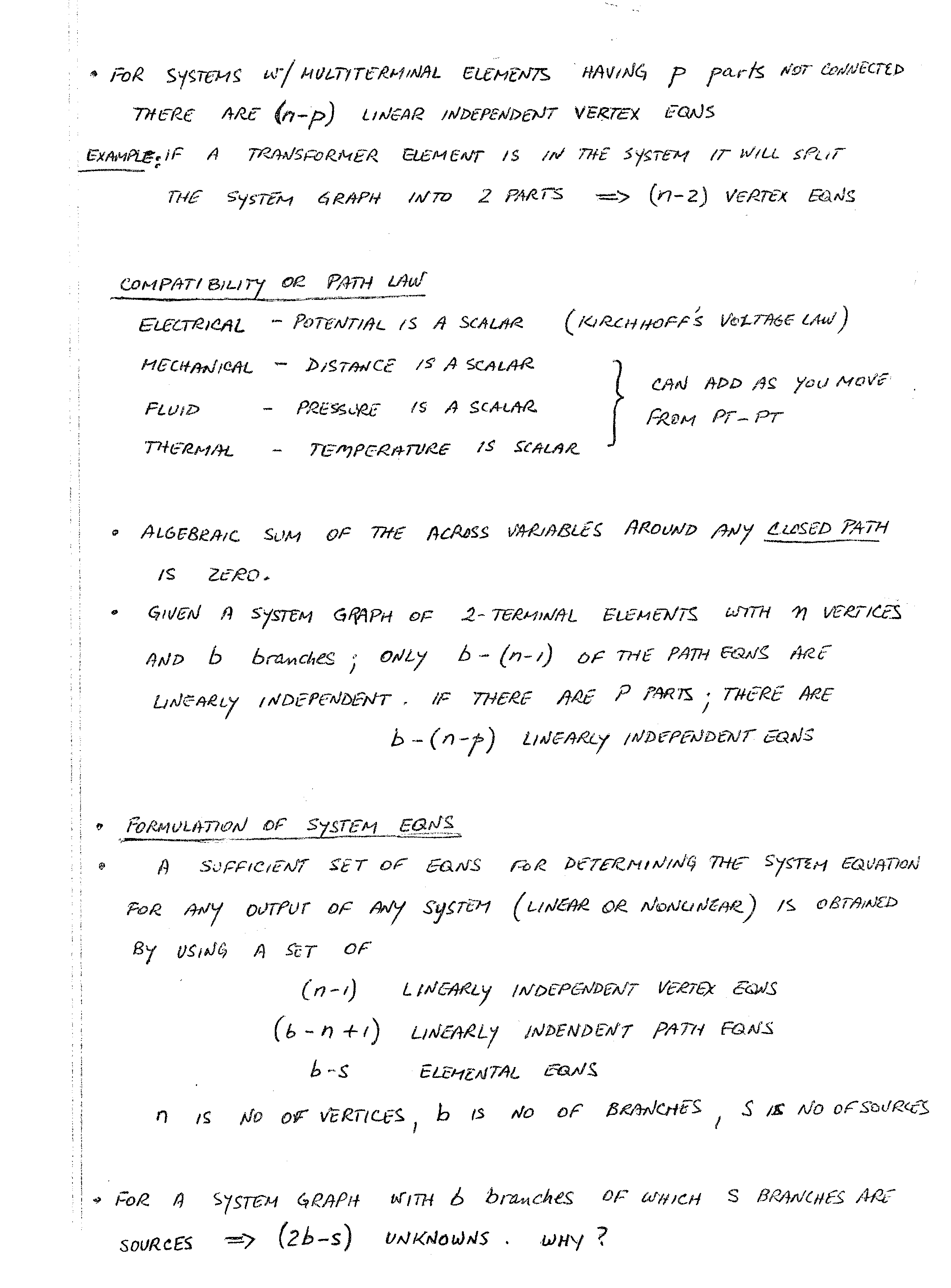
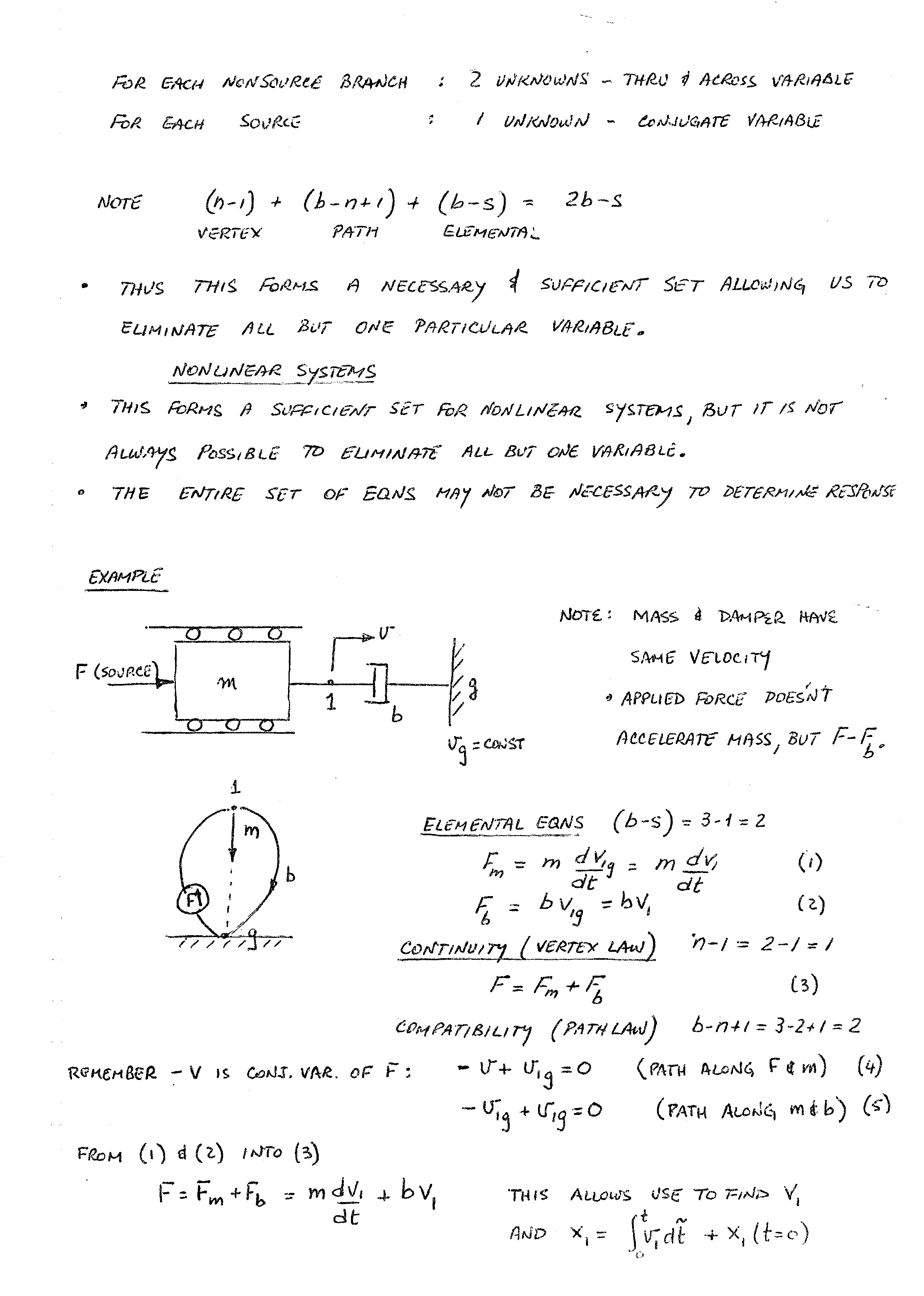
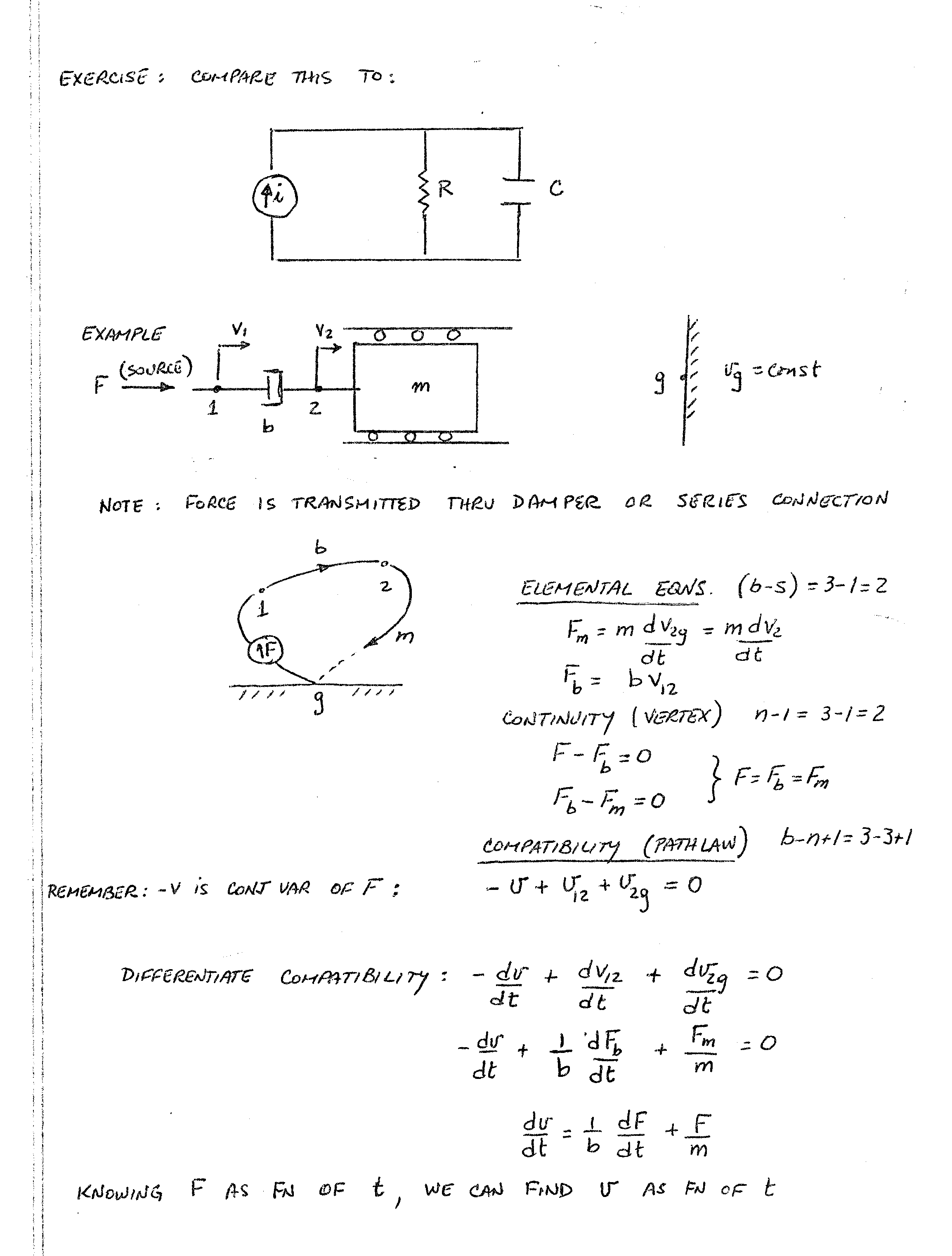
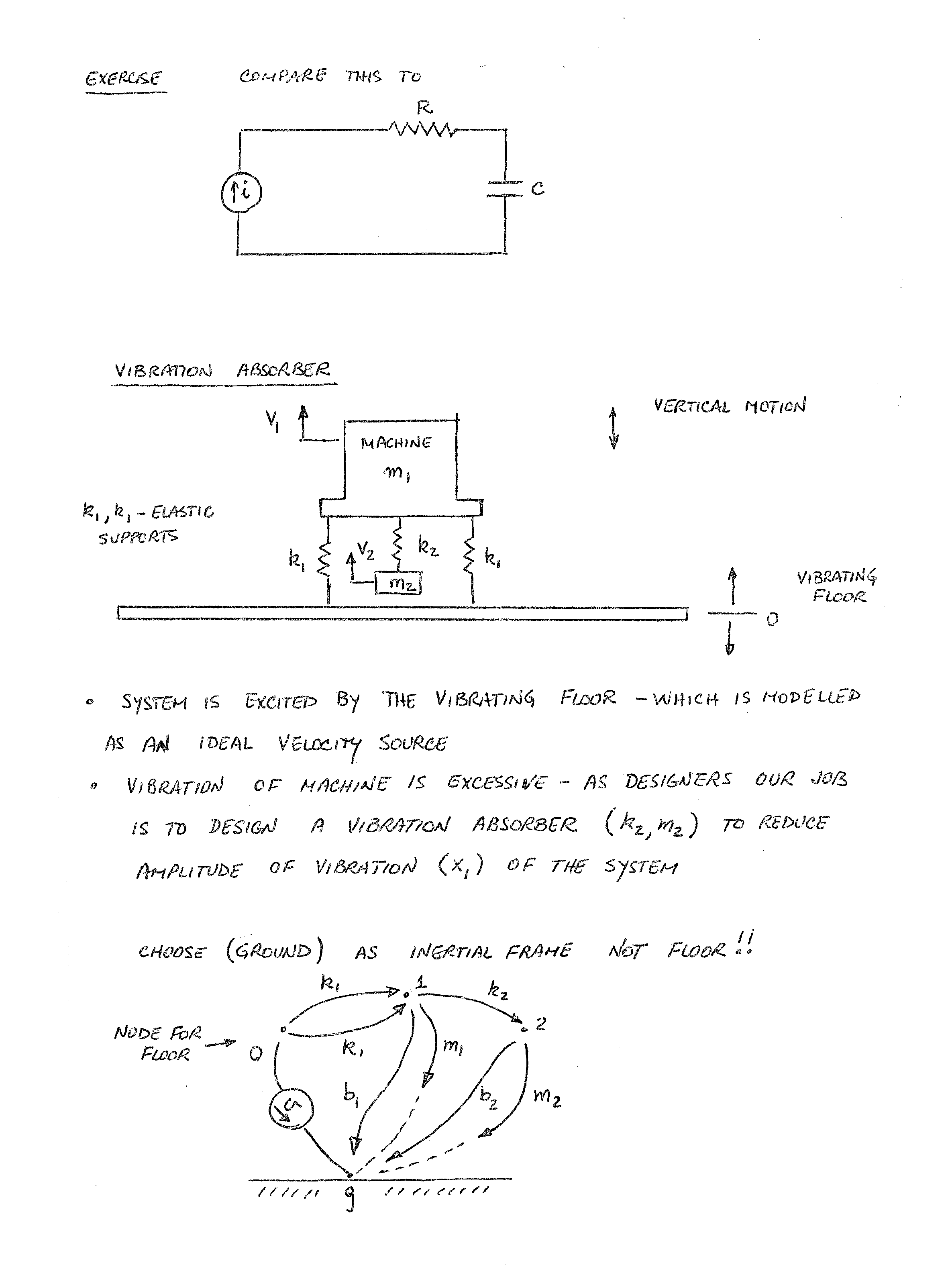
Here is Lecture 9 video: we did two problems, one forced undamped and one forced damped vibration problem. We then began the topic of system dynamics by defining the through and across variables, the elemental and constitutive equations, the ideal and pure element. Here are the pages that go with the last part of the lecture: page 9, page10, page11, and examples,

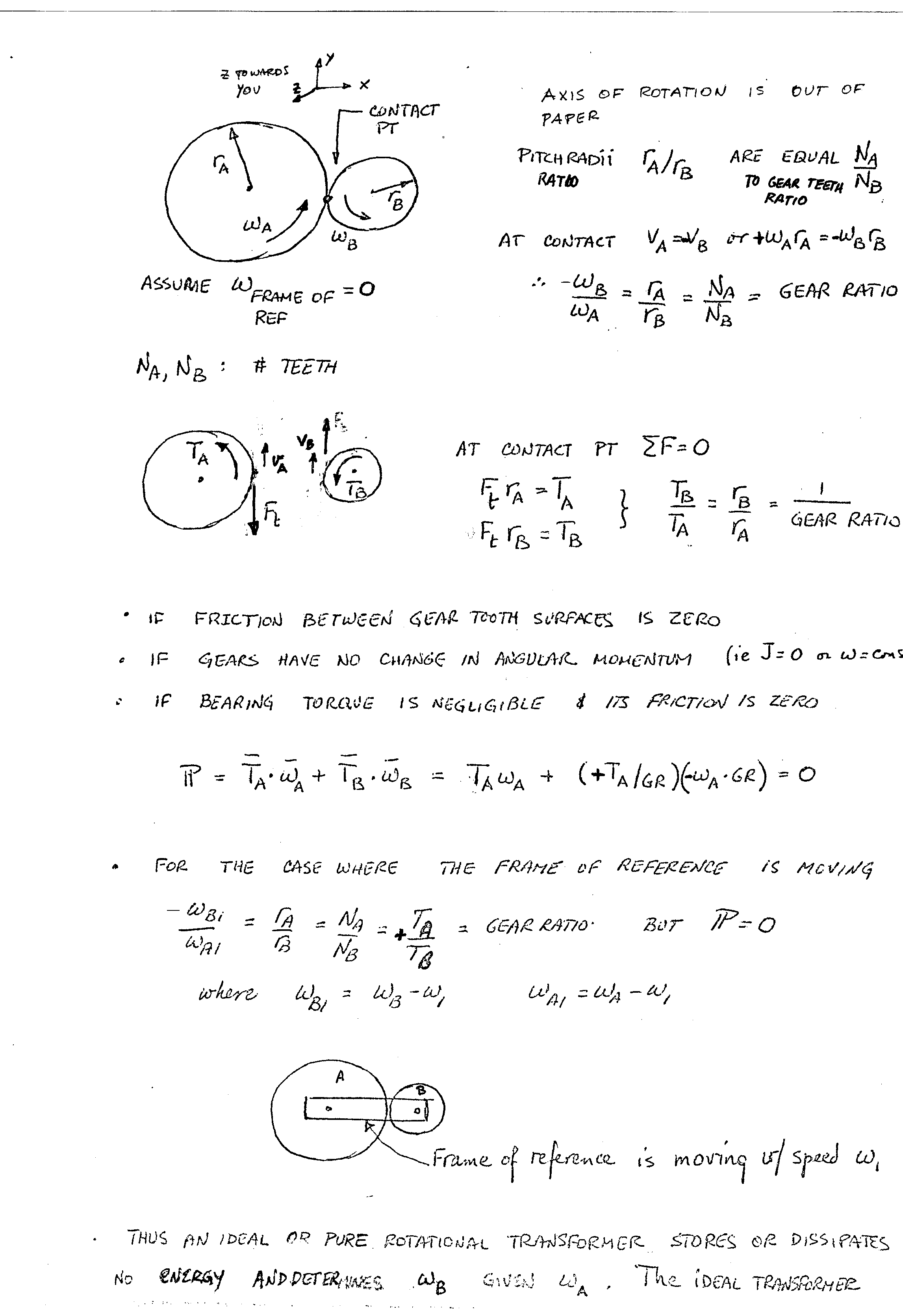
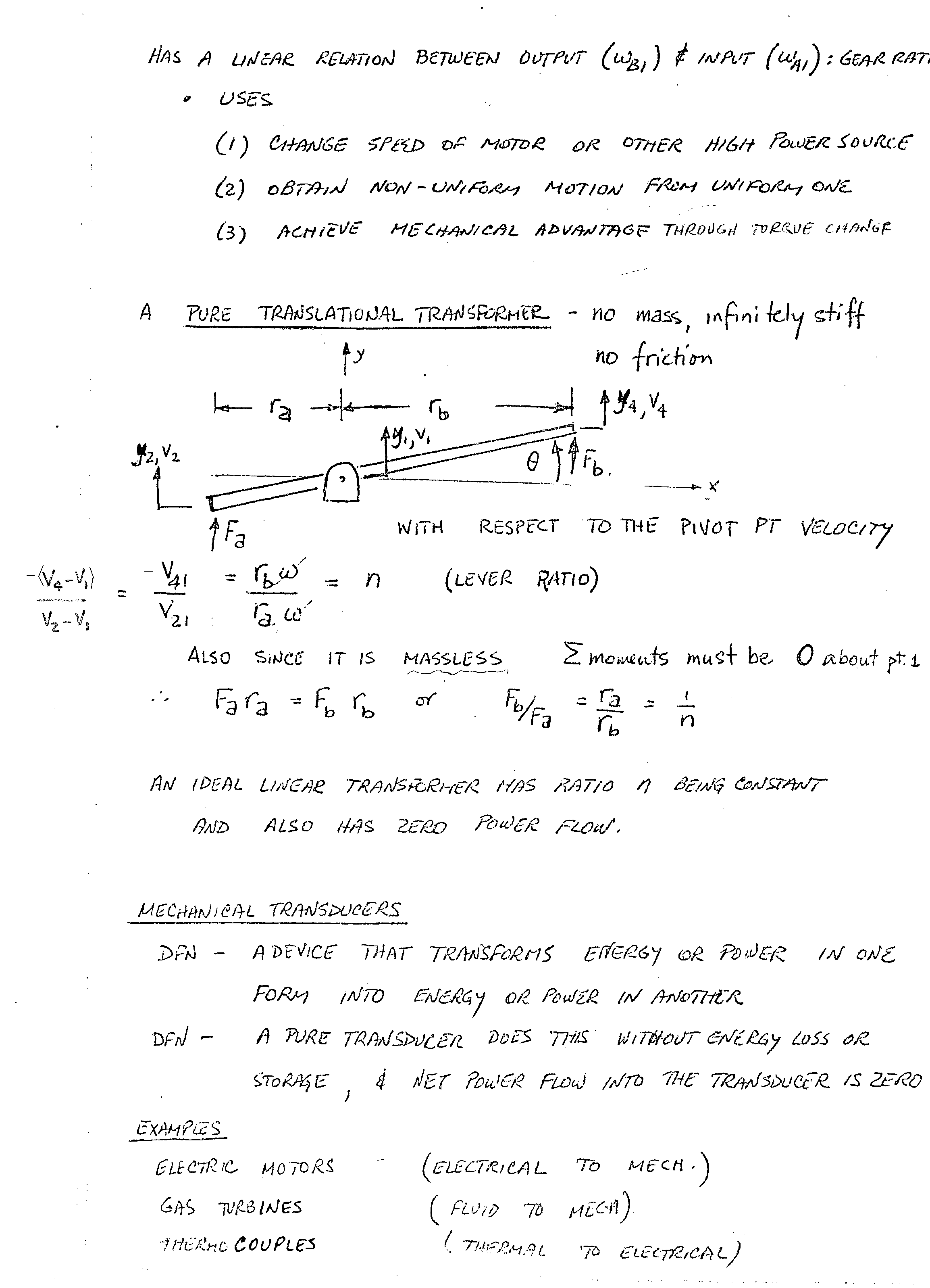
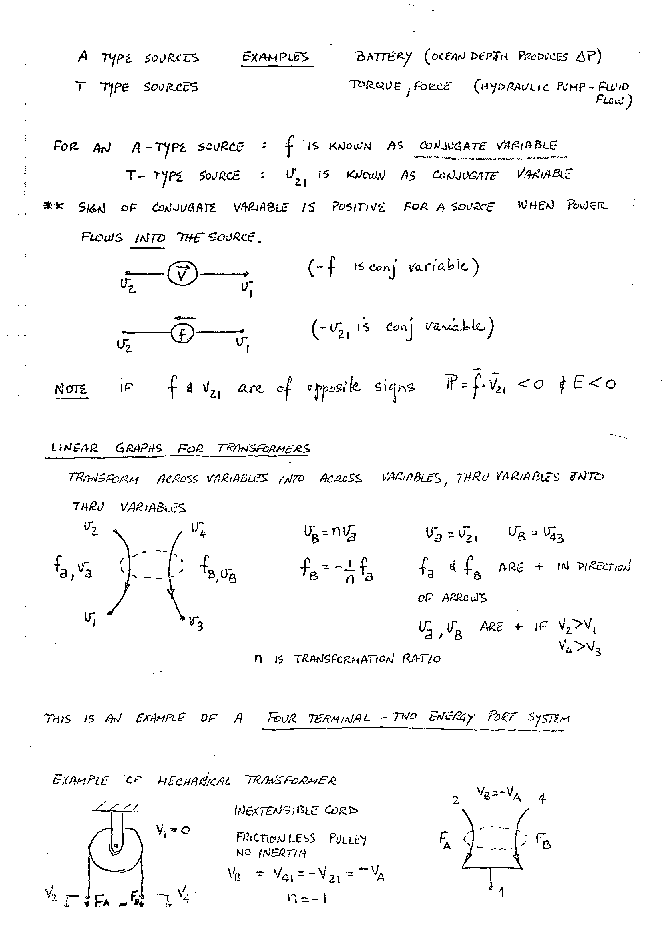
Here is the material that goes with Lecture 10 video on rotational mechanical systems and transformers, both rotational and linear mechanical: page12, page 13, page 14, page 15, page 16.

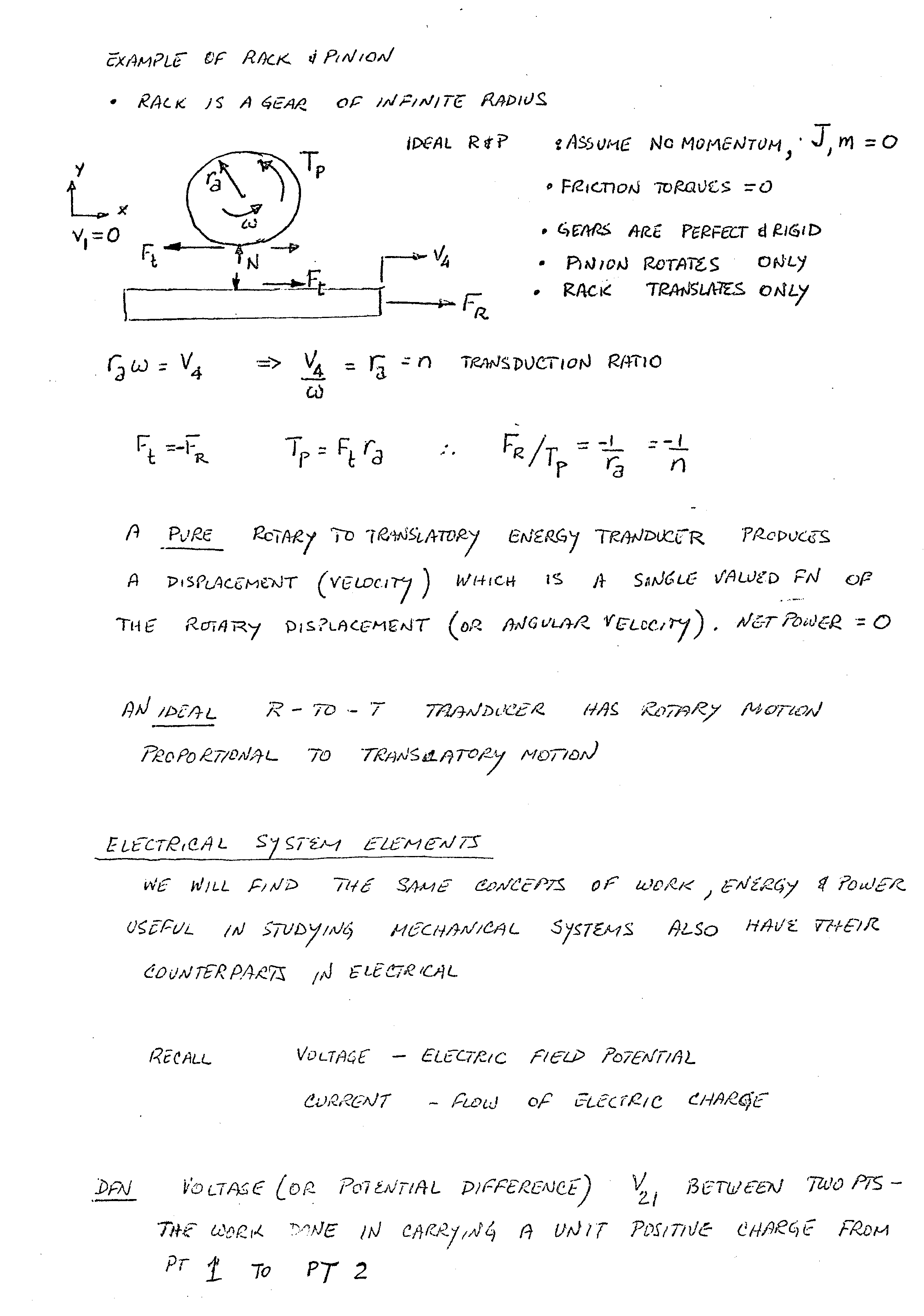
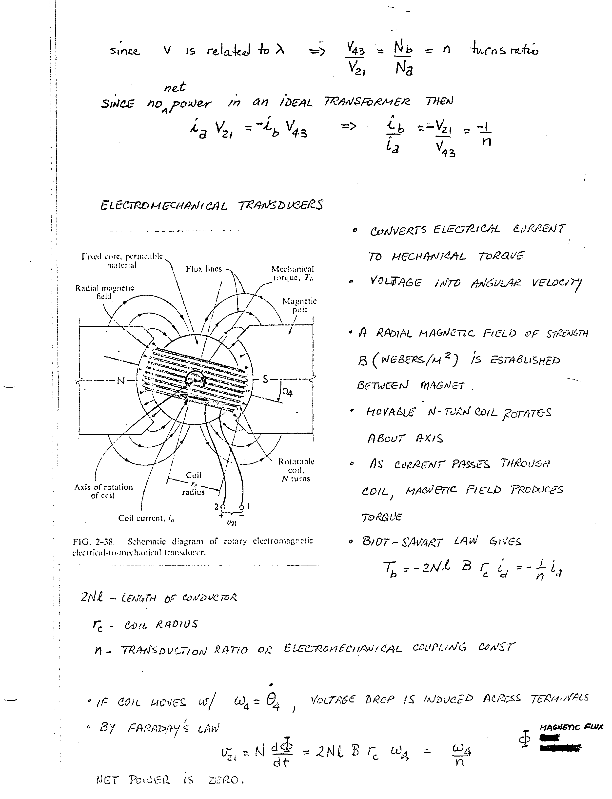
Here is the material that will go with Lecture 11 video on transformers including rack and pinion: page 16, page 17, and continues on page 18, page 19, page 20, examples with electrical elements including transformers and transducers, examples with electrical elements 2, page 21

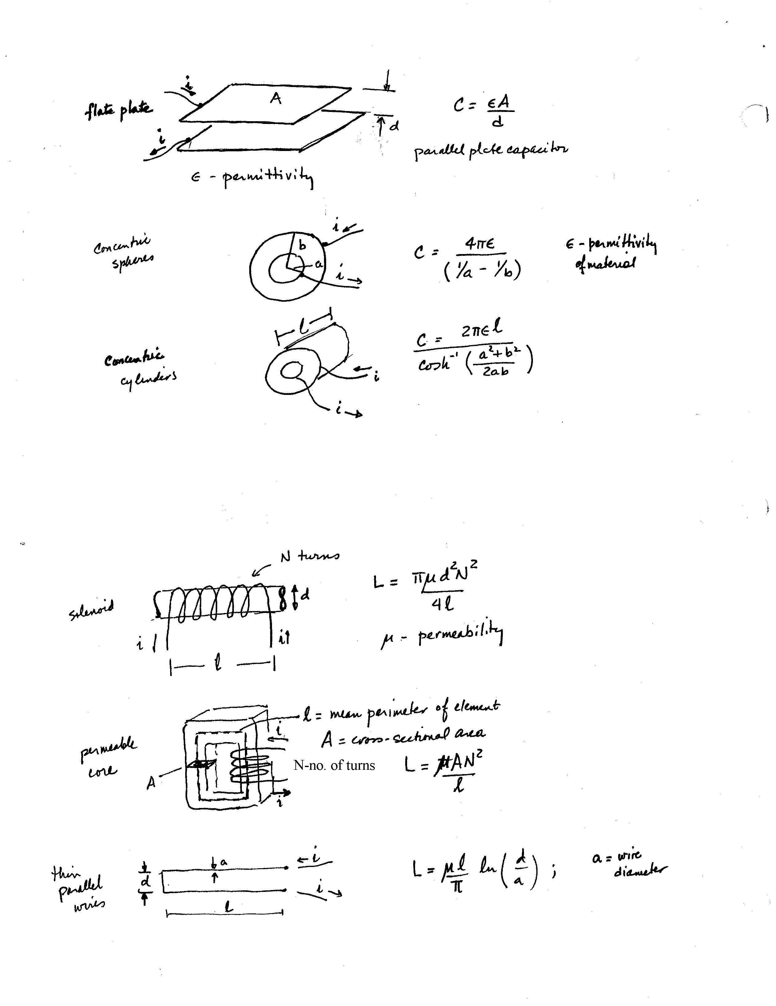
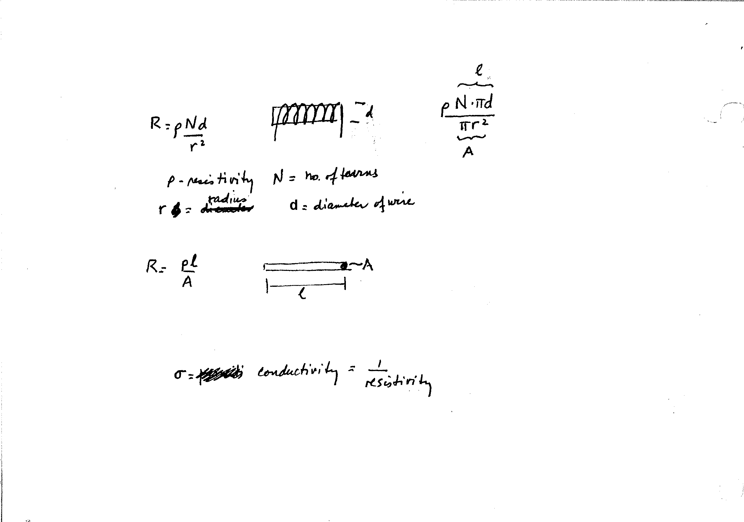
The information on pgs 17-21 of Rowell and Wormley’s book deals with electrical elements: capacitors, inductors and resistors. They are like electrical “masses”, “springs” and “dampers”. The material will not be covered in depth in class but you will be responsible for it. I will skim over the material to cover the main elements, transformers and transducers. Just note the similar way we can describe electrical elements.

Start reading chapter 6 on transducers in one energy domain (transformers) and transducers in multi energy domains (transducers)

Work on the following problems 1.1, 1.4, 2.2, 2.4 from your books not the notes. Solutions will be posted next Monday Sept 26.

We will have our first quiz on Monday Sept 26 on vibrations related to the three handouts (free and forced vibrations, vibrations with and without damping). You are allowed 2 8.5x11 inch pages of formula sheets only. This quiz will cover materials from videos 1-9.

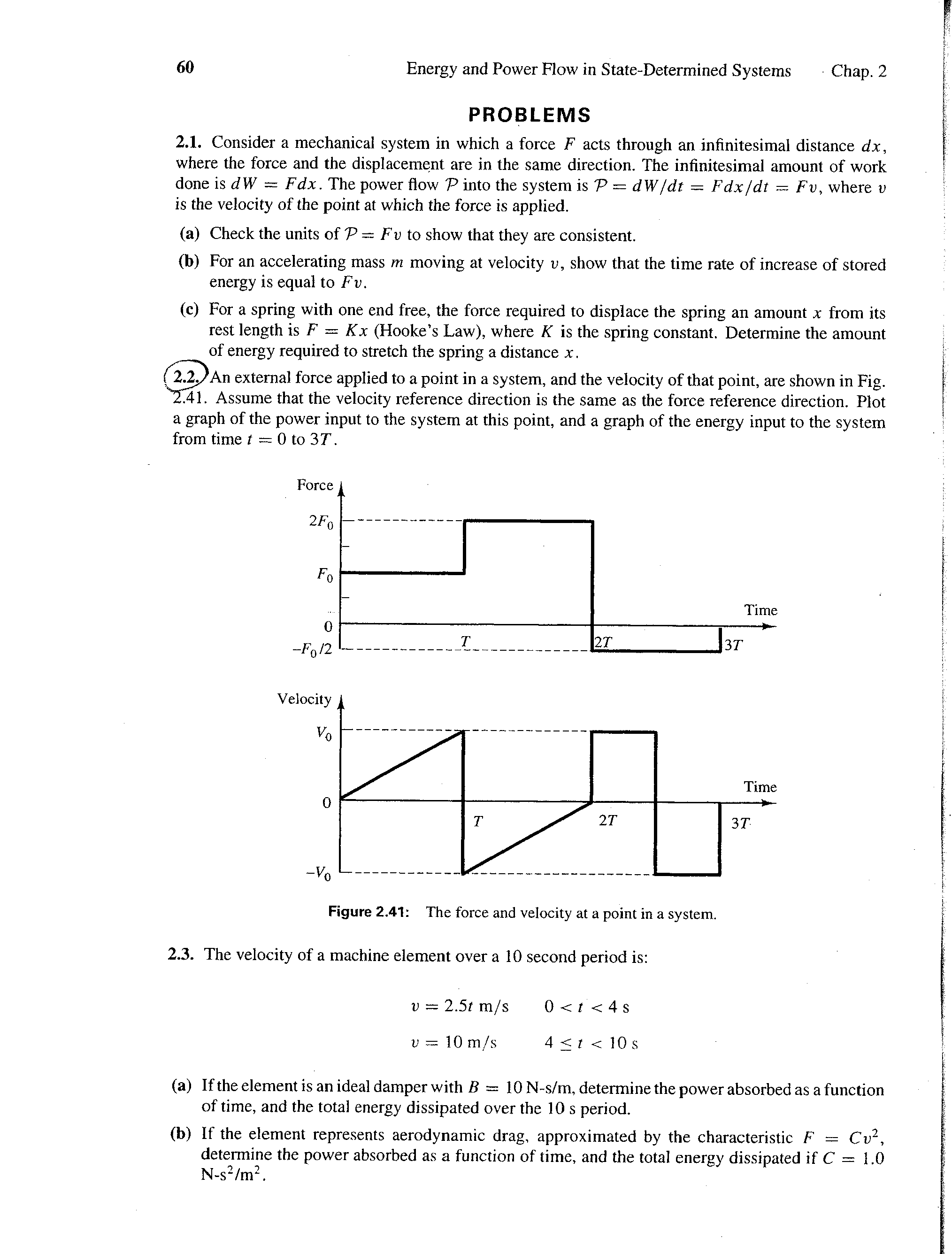
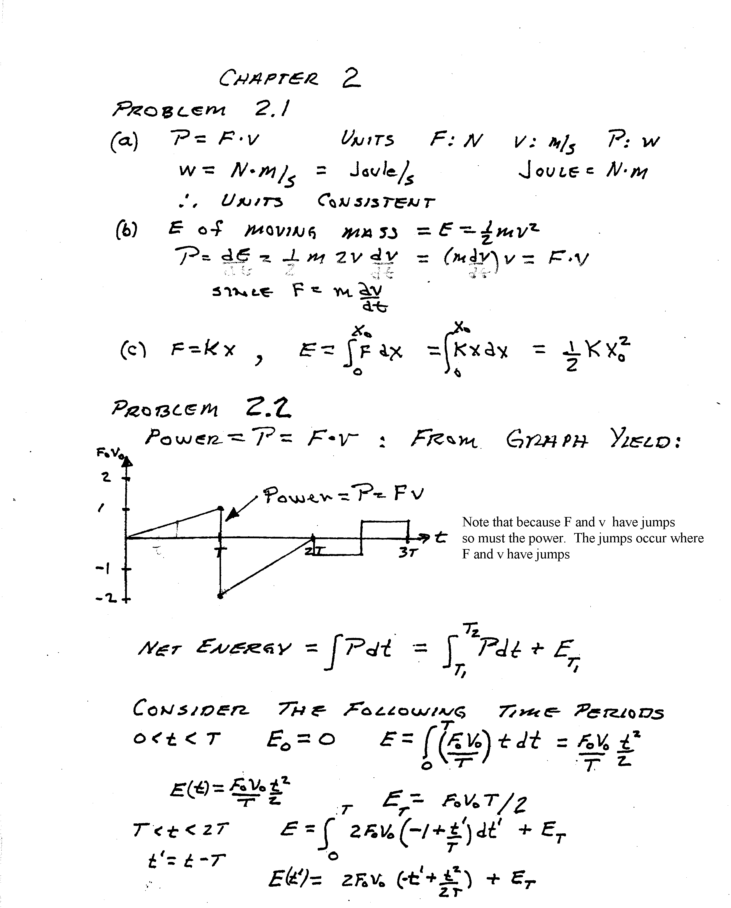
Here are problems 2-4, 2-6 and 2-7 Note that more comments about 2-7

Are found on the top of the page for problem 2-13

Here are problems 2-17, 2-18, 2-19

Here are problems like 2-28, 2-38

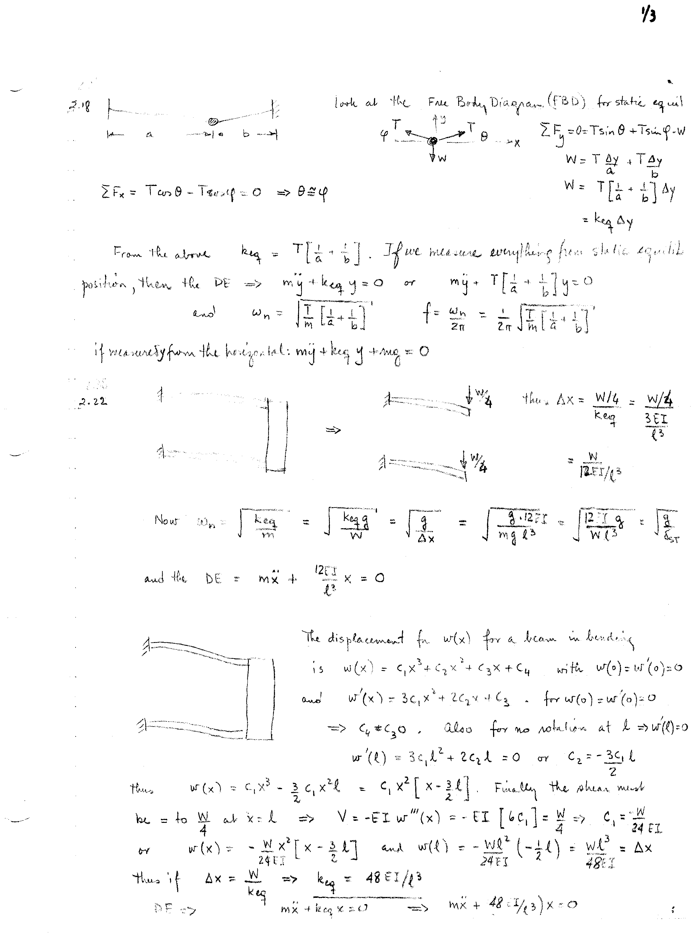
Here is the rest of 2-38, and problems 2-68, 2-79

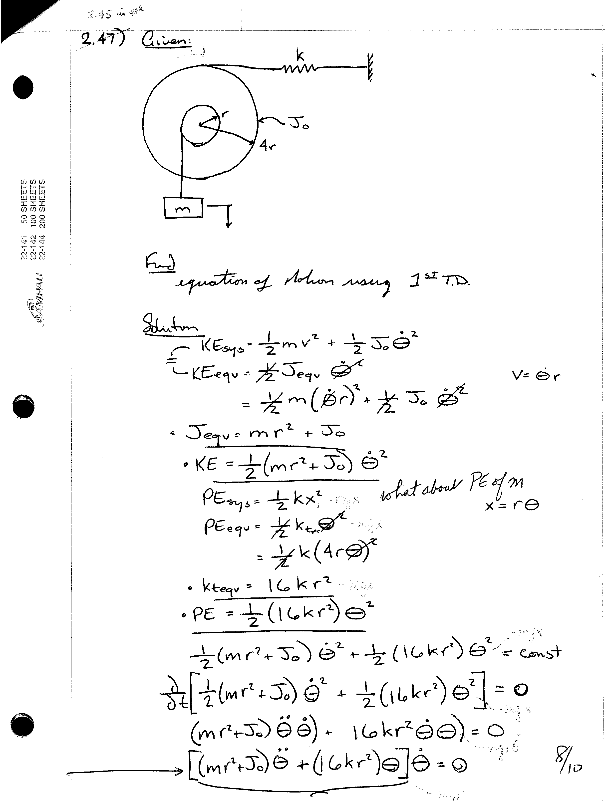
Here is problem 2-45

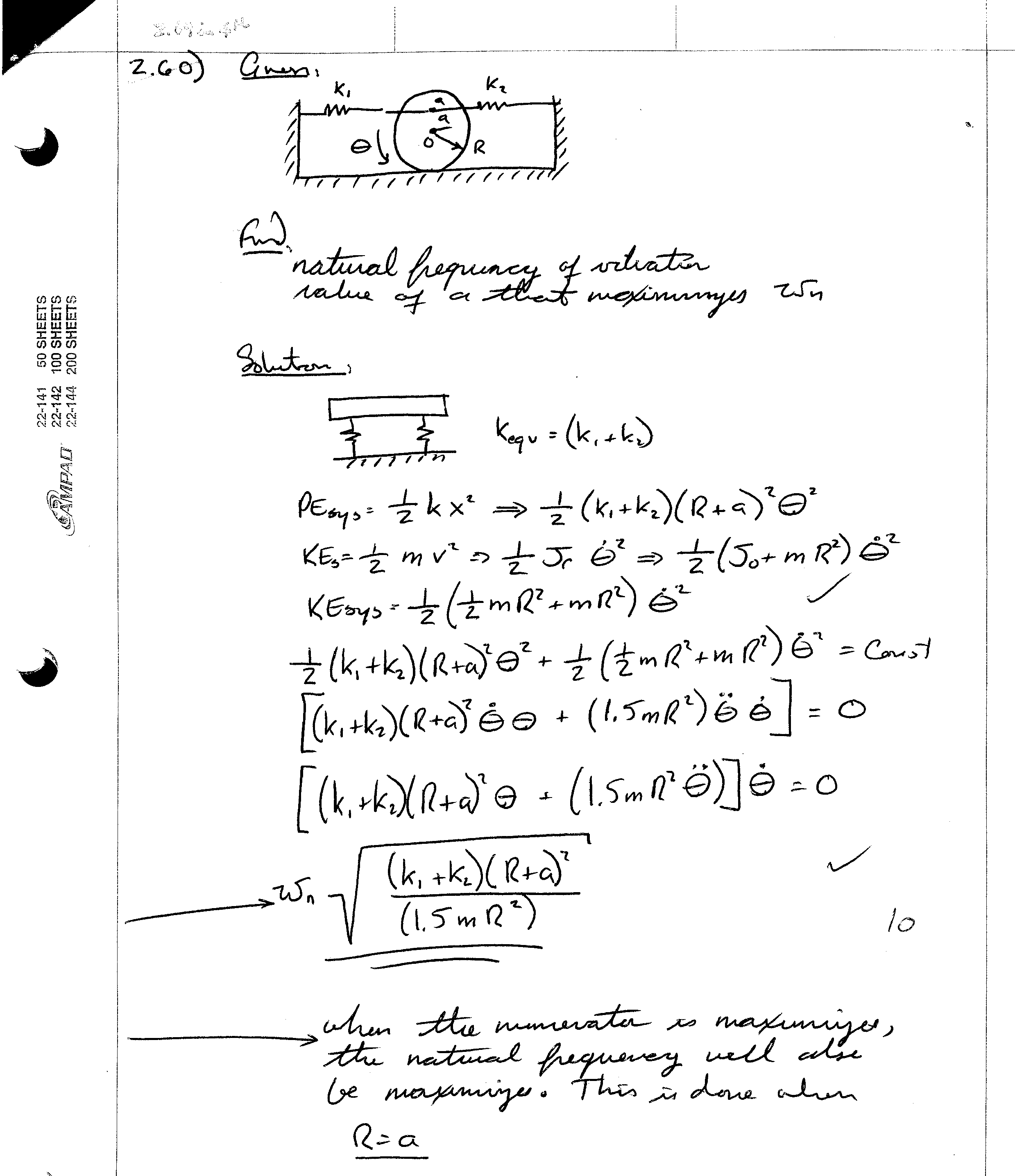
Here is problem 2-60

Here, the second problem is like problem 2.80

Here are problems the first two are like 2.83, 2.97

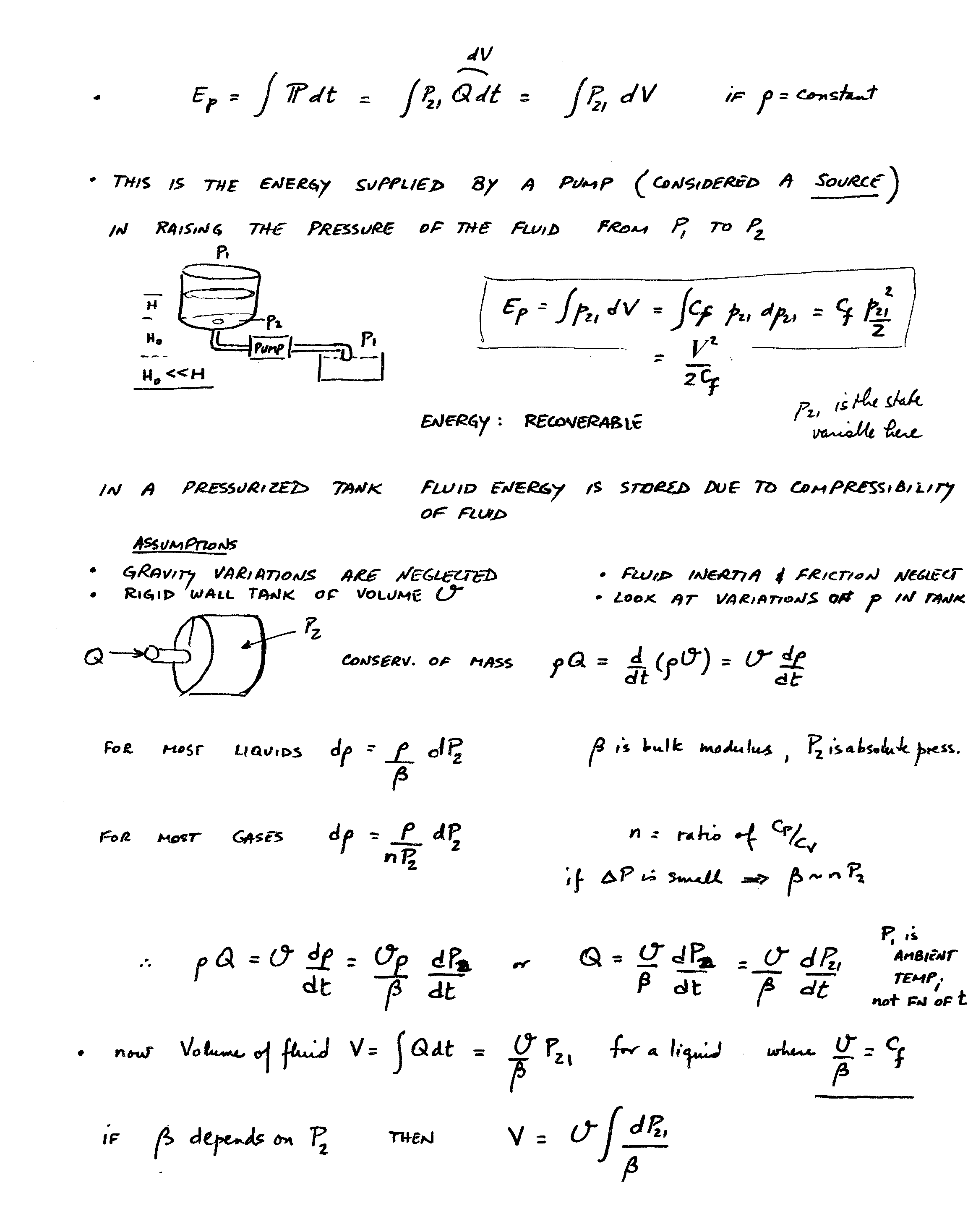
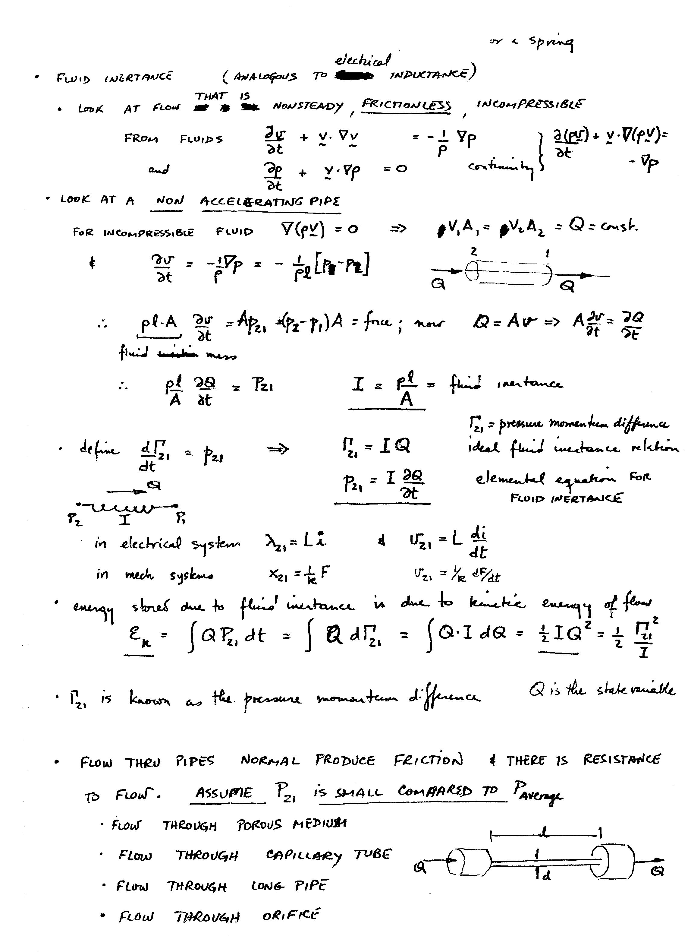
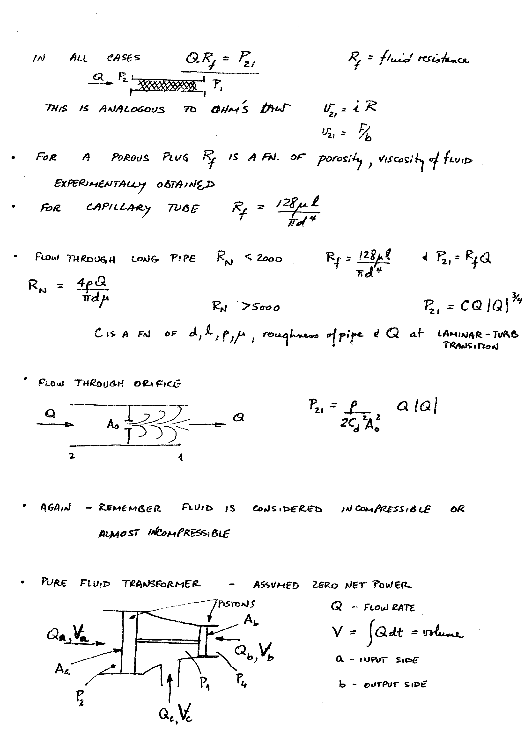
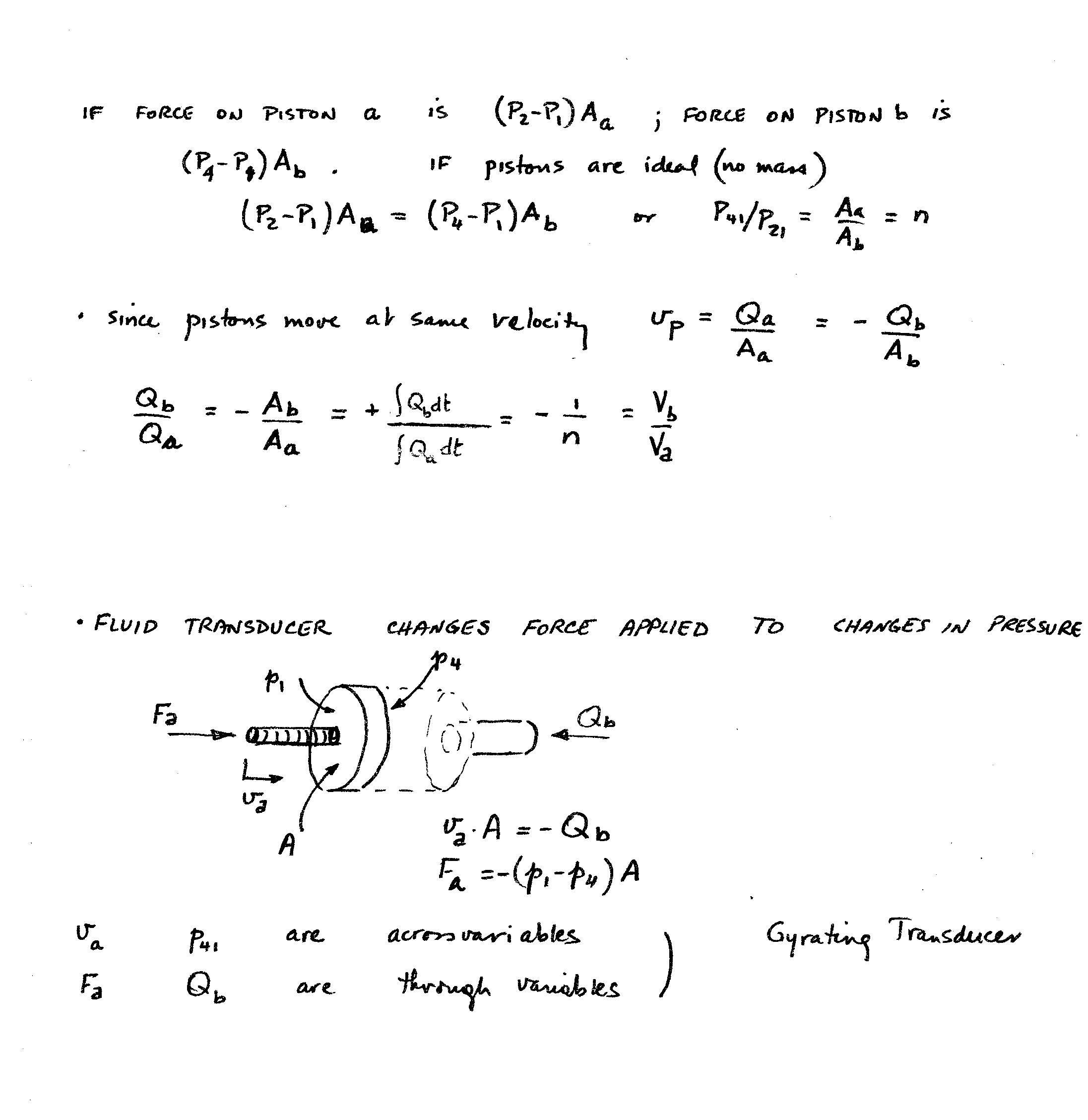
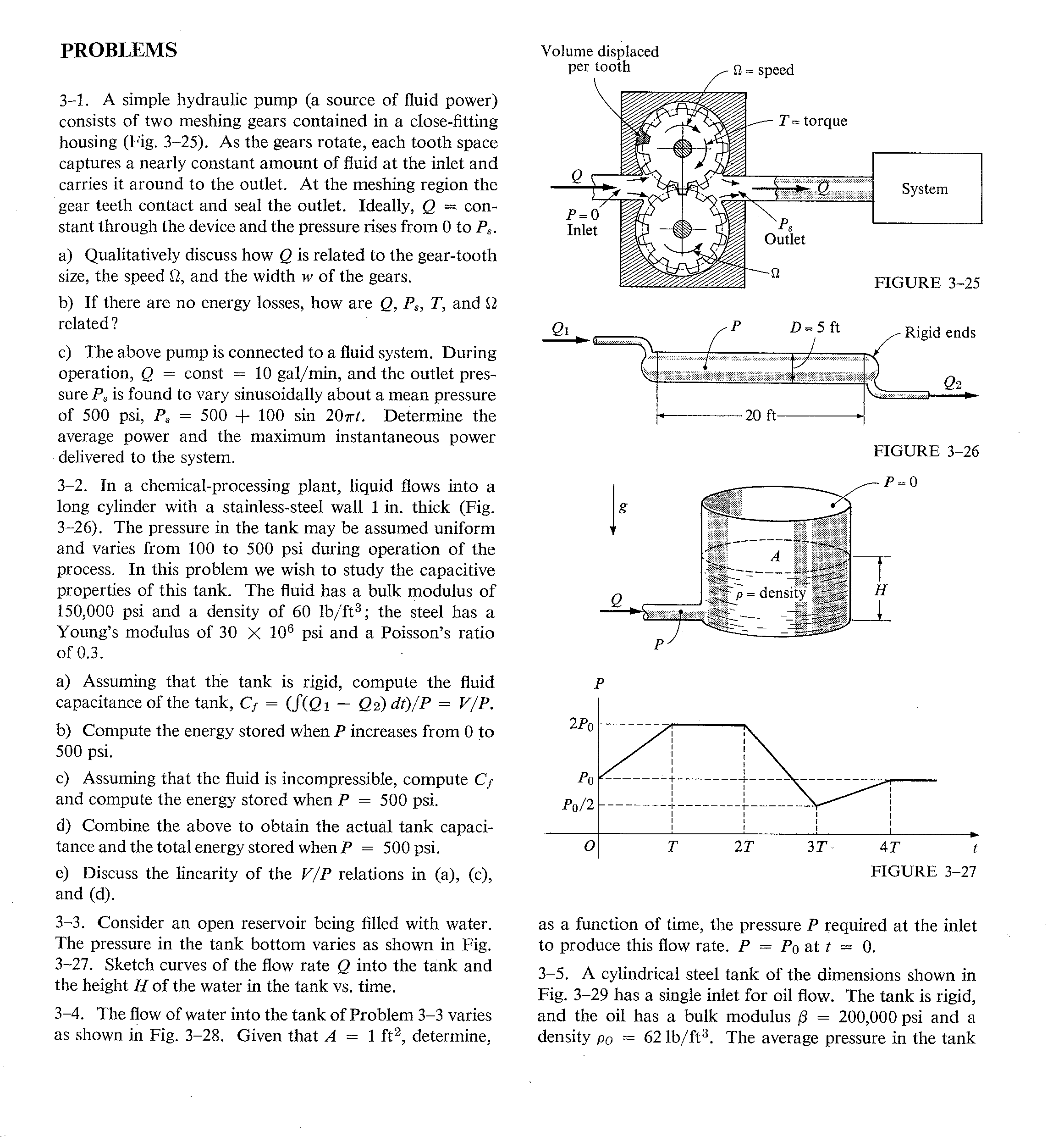
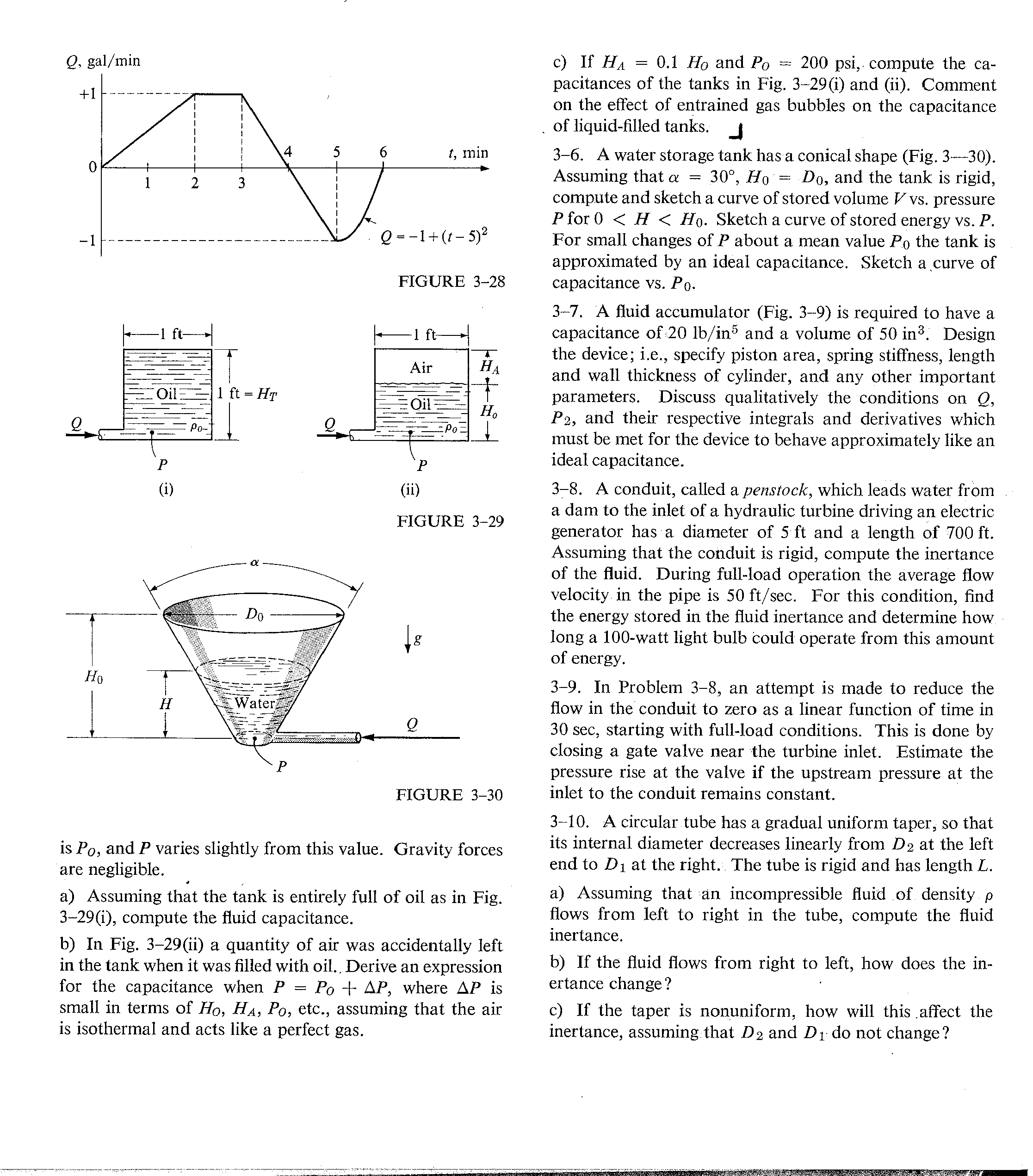
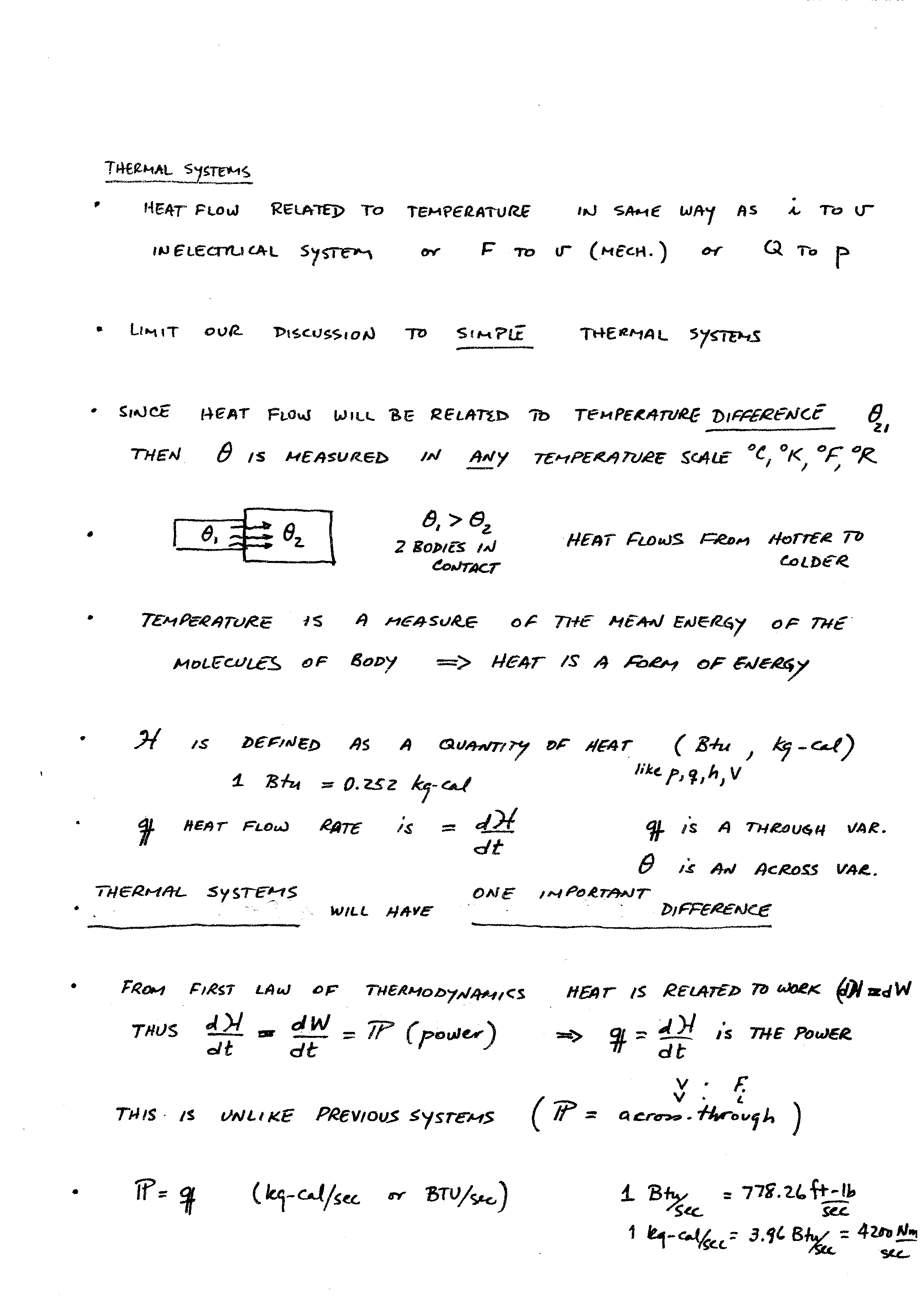
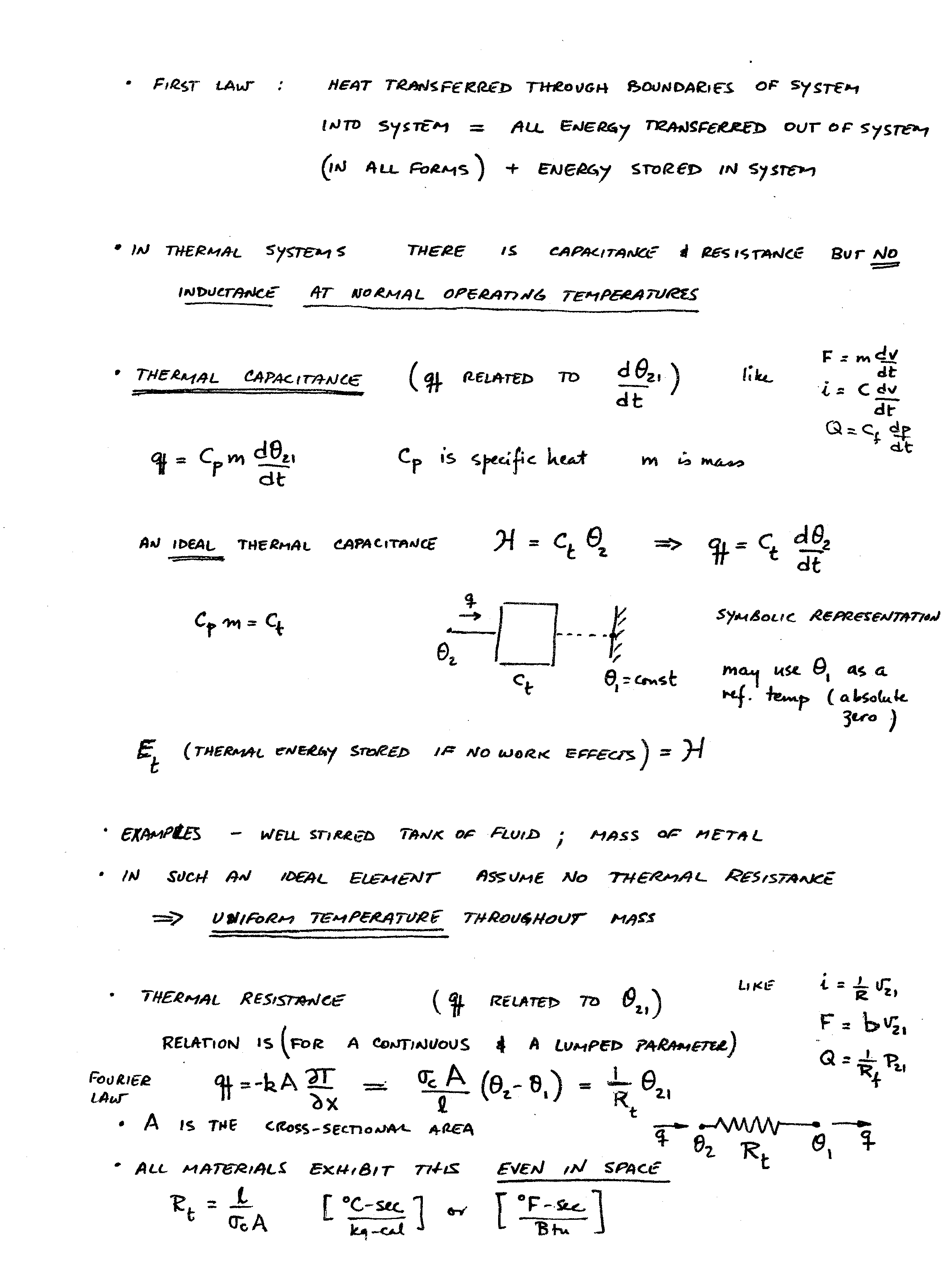
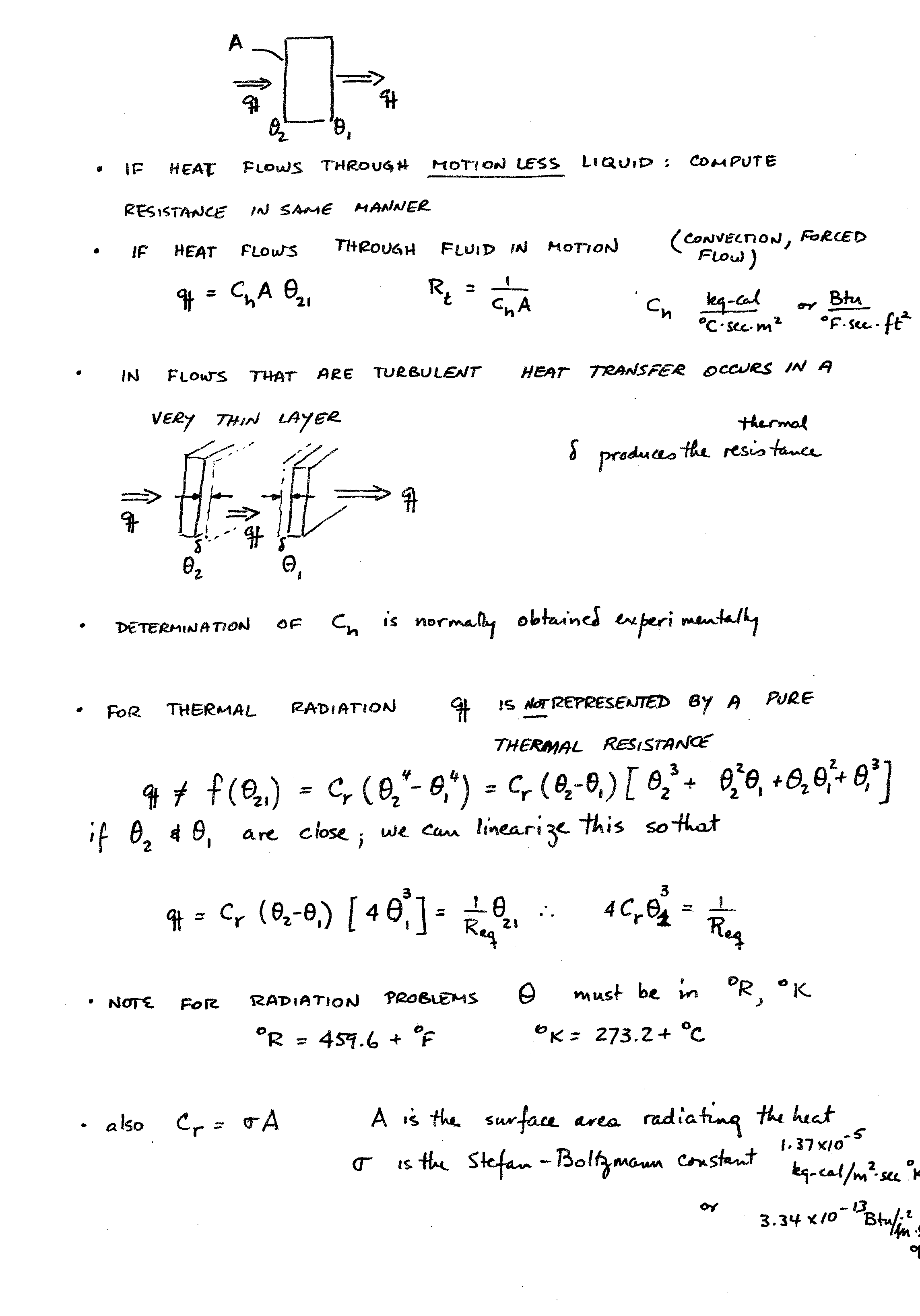
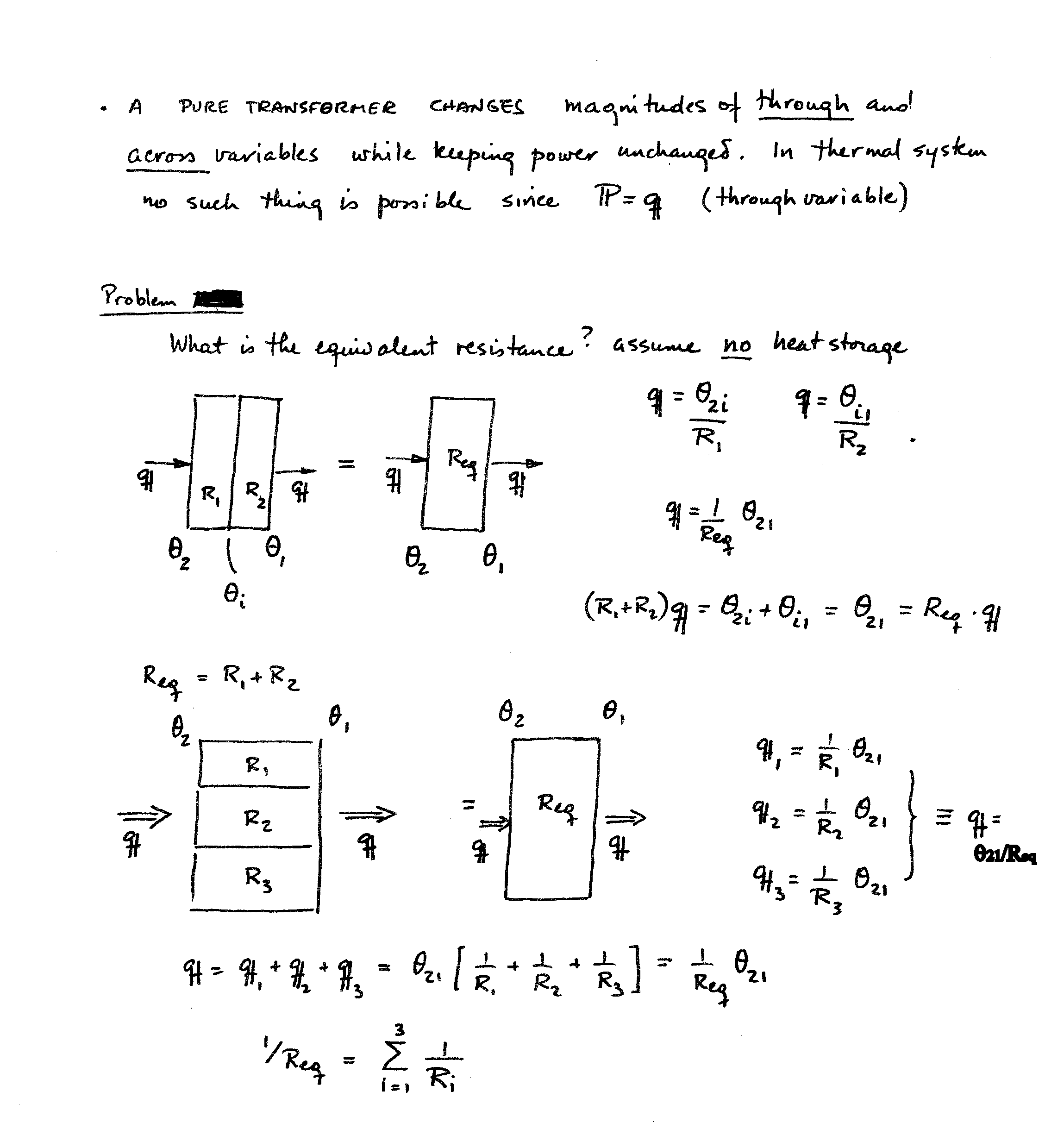
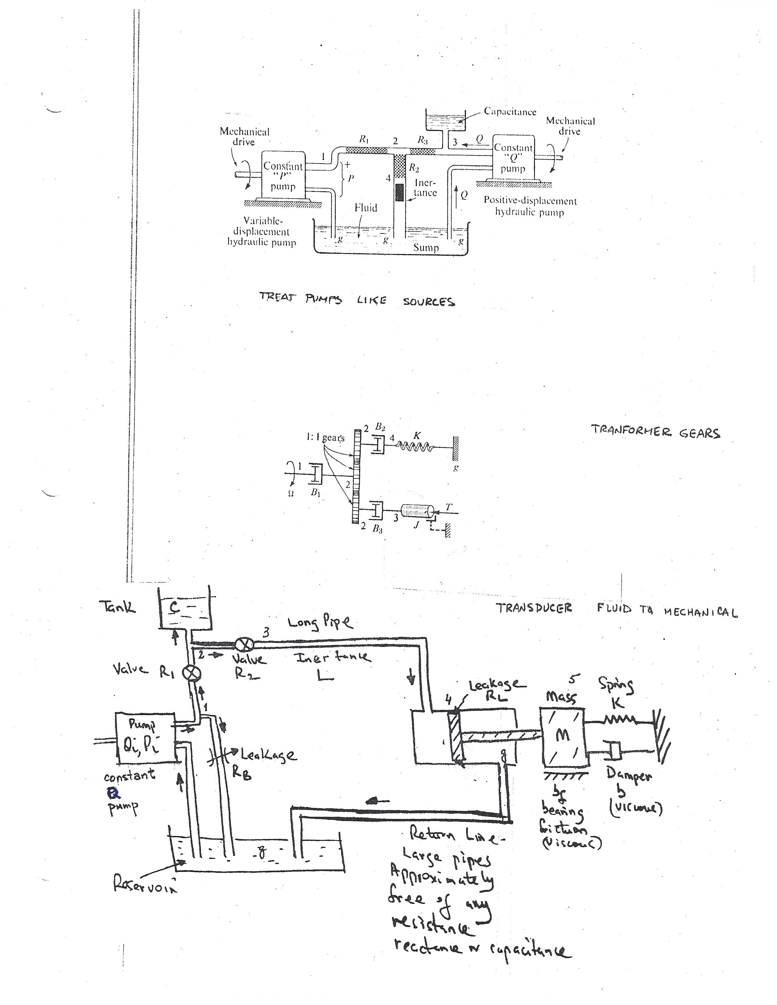
Here are the pages that go with Lecture 12 on Fluid systems: page 22, page 23, page 24, page 25, page 26, page 27, The last two pages deal with fluid transformers and transducers

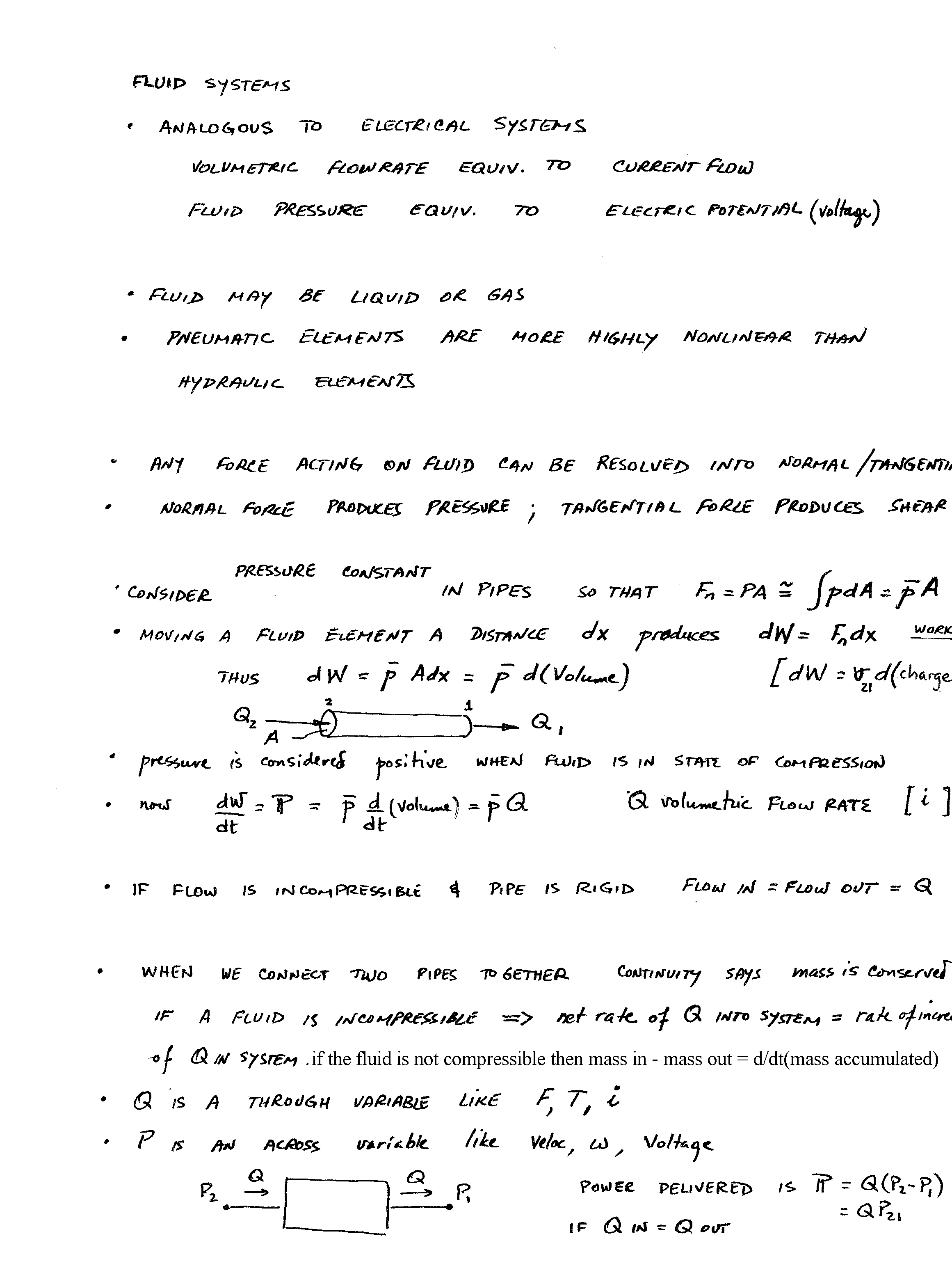
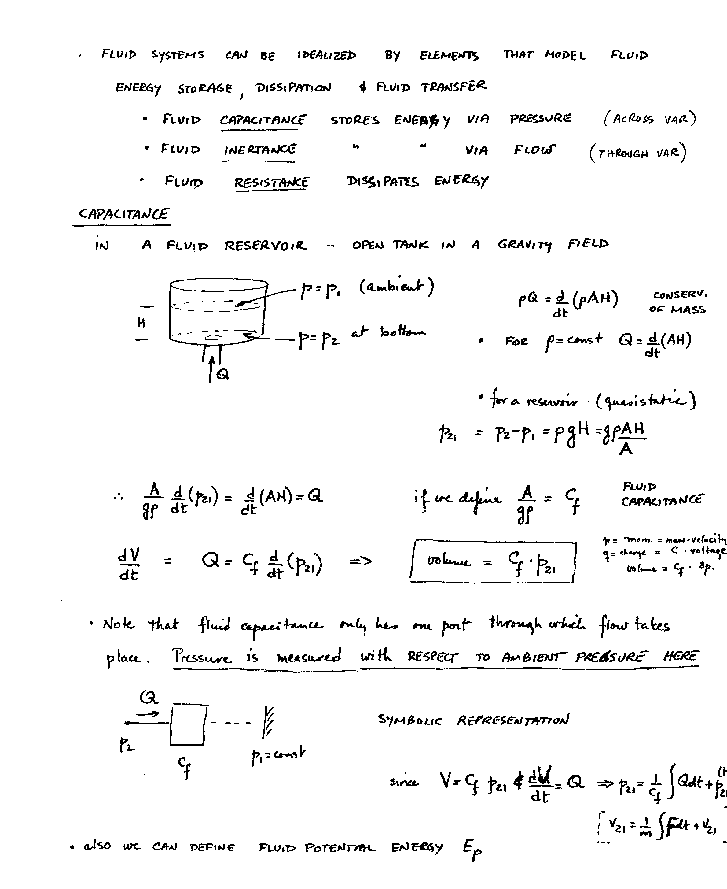
Lecture 13: quick review of the material to this point. First exam is announced again for Monday September 26

Lecture 14: exam on vibrations of mass-spring, mass-spring-dashpot systems with and without forcing functions.

Here are the Problems 1.1, 1.4, 2.2, 2.4 and the solutions: problem 1, problem 2a 2b, problem 3a 3b, problem 4

Here is the material that will go with Lecture 15 video: page 26, page 27, page 28, page 29, page 30,

Here is the material that will go with Lecture 16 video for 9/30: page 30, page 31, page 32, page 33, page 34, example solution

Please do problems 4.1, 4.2, 4.5 and 4.11 in your books. They are due on October 10, 2011.

Here is the material that goes with Lecture 17 10/3video: page 36, page 37, page 38, page 39, page 40, page 41, page 42

Here is the material that goes with Lecture 18 10/3 video: page 42, page 43, page 44, page 44solution,, page 45-46 examples, page 45-46solns

Here is the material that goes with Lecture 19 10/7 video: page 47, page 48, page 49, page 50, and page 51,

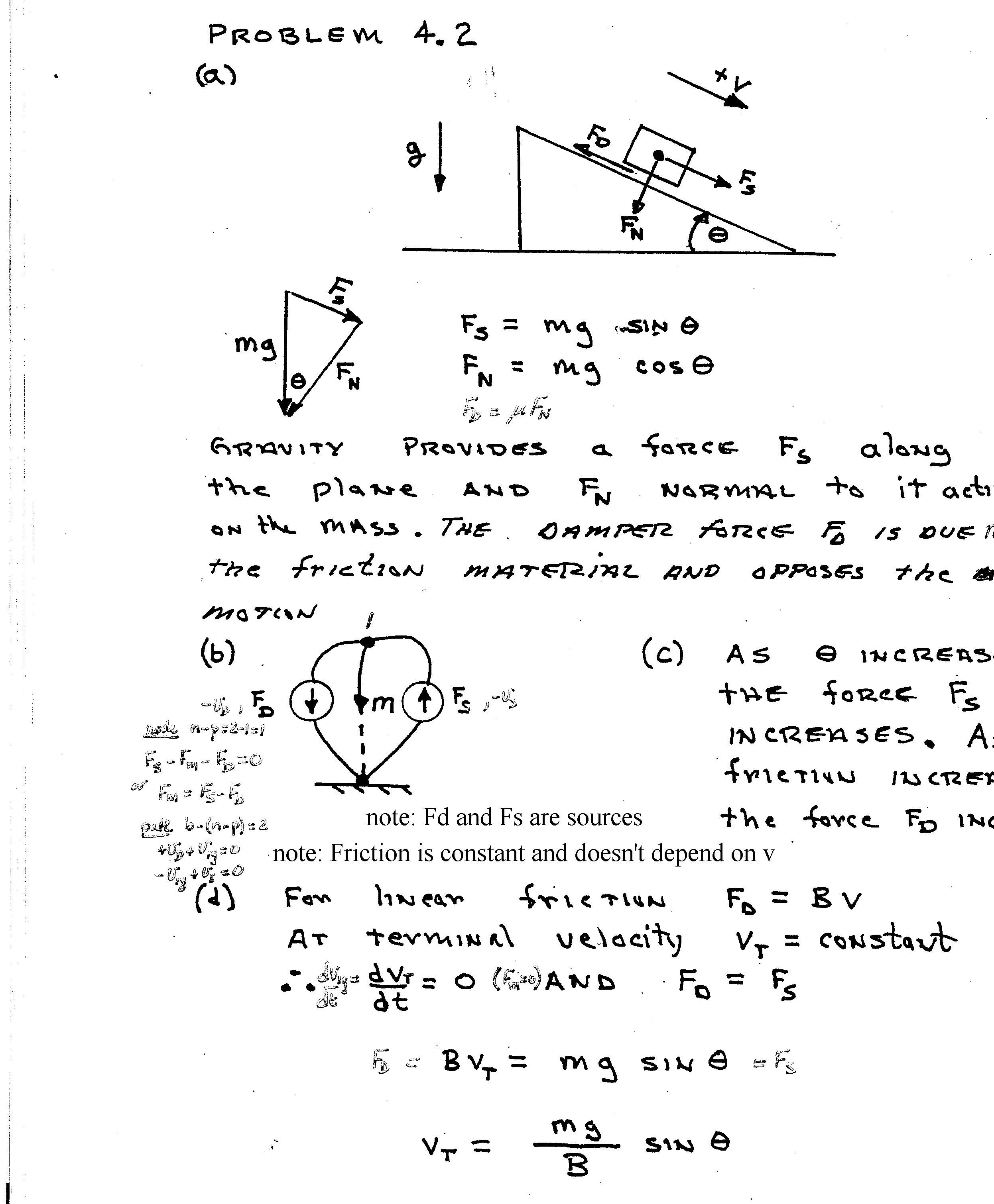
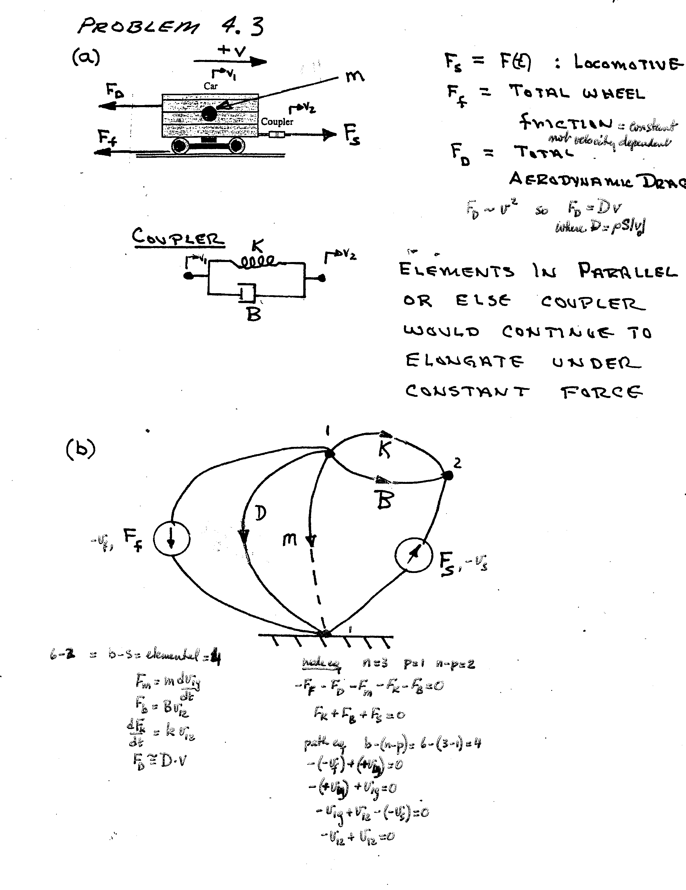
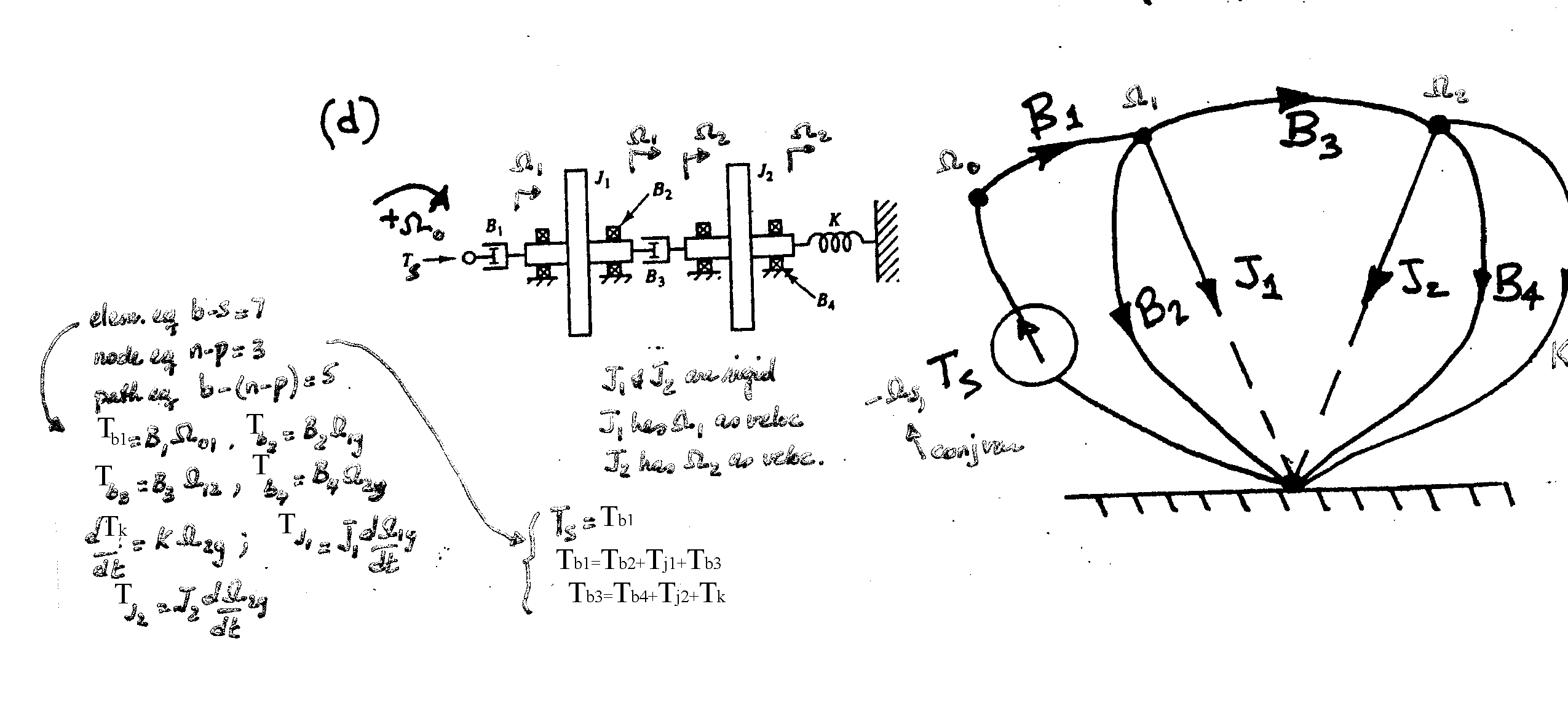
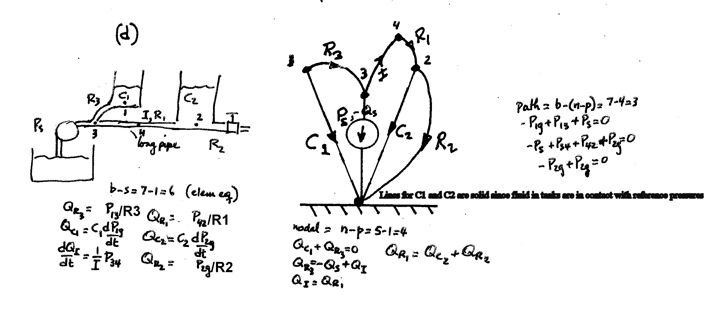
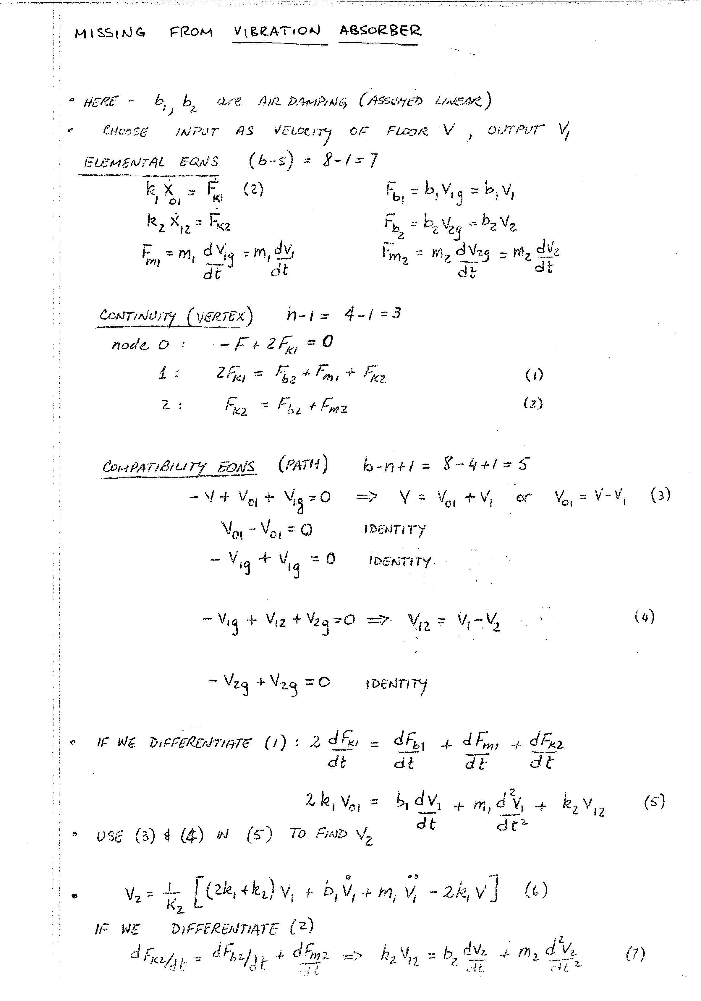
HERE I provide you with the solutions to PROBLEMS 4.2, 4.3, 4.6d and 4.11d

Here is the material that goes with Lecture 20 10/10 video: page 51, page 52, page 53, page 54,

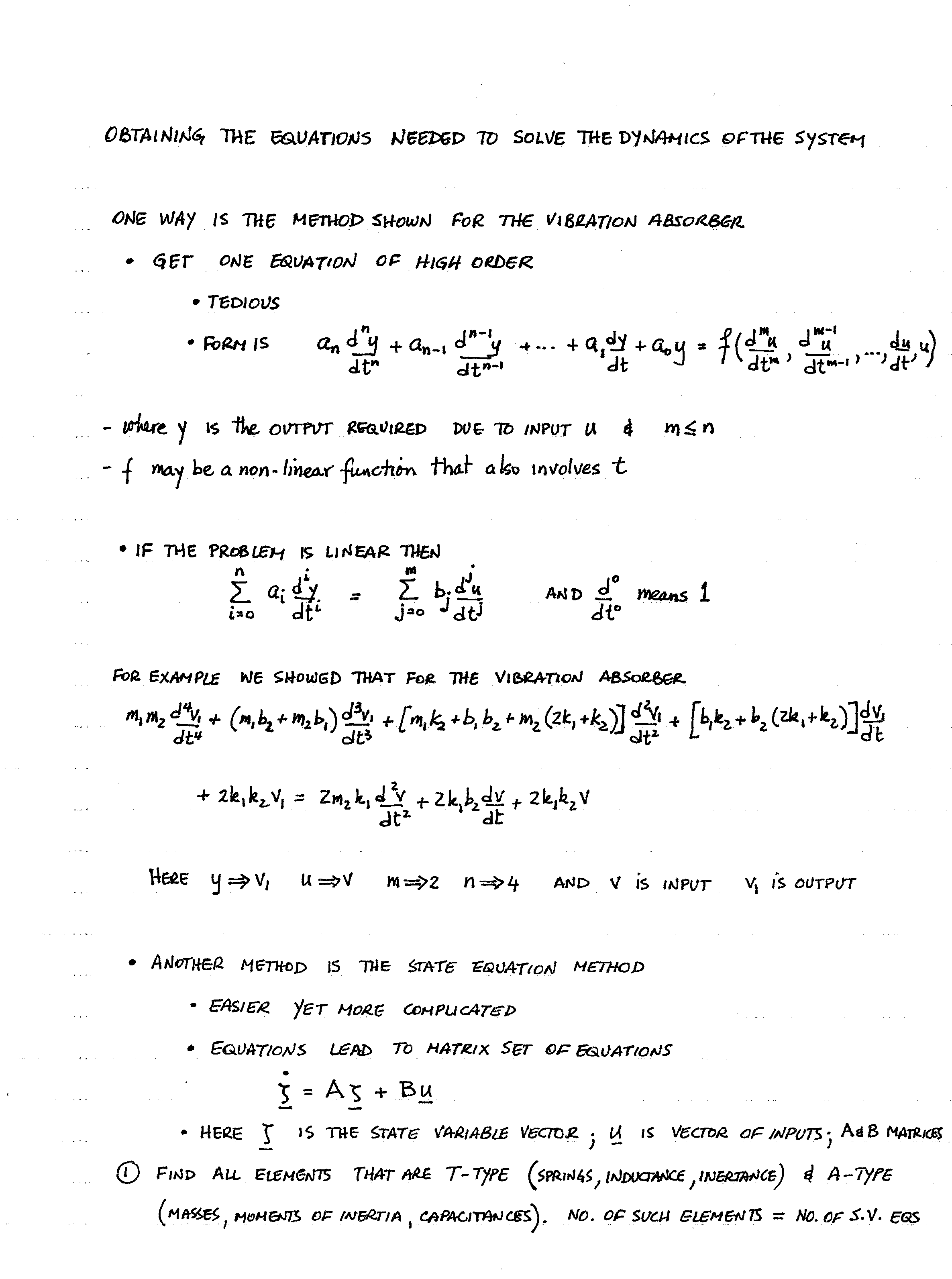
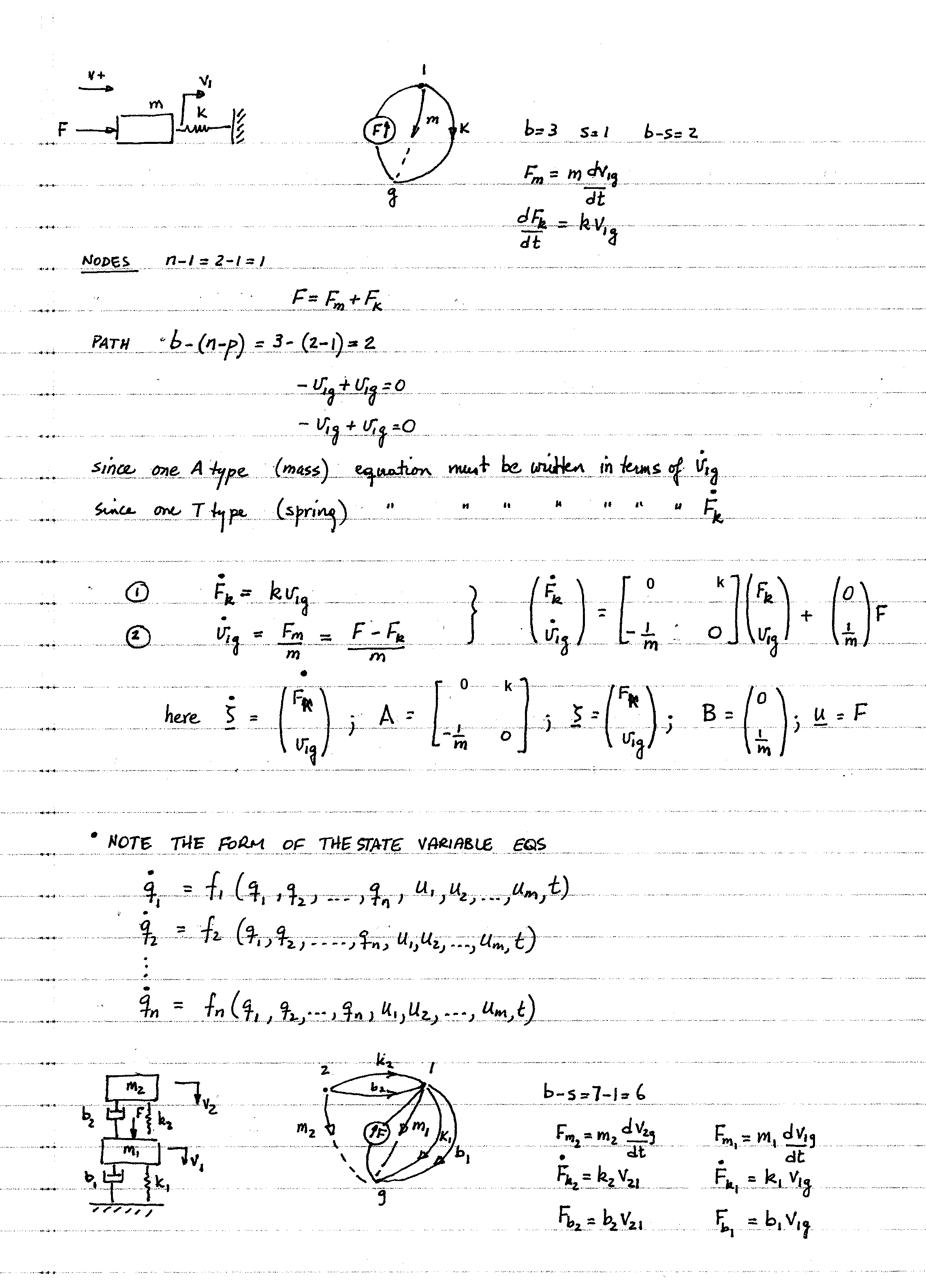
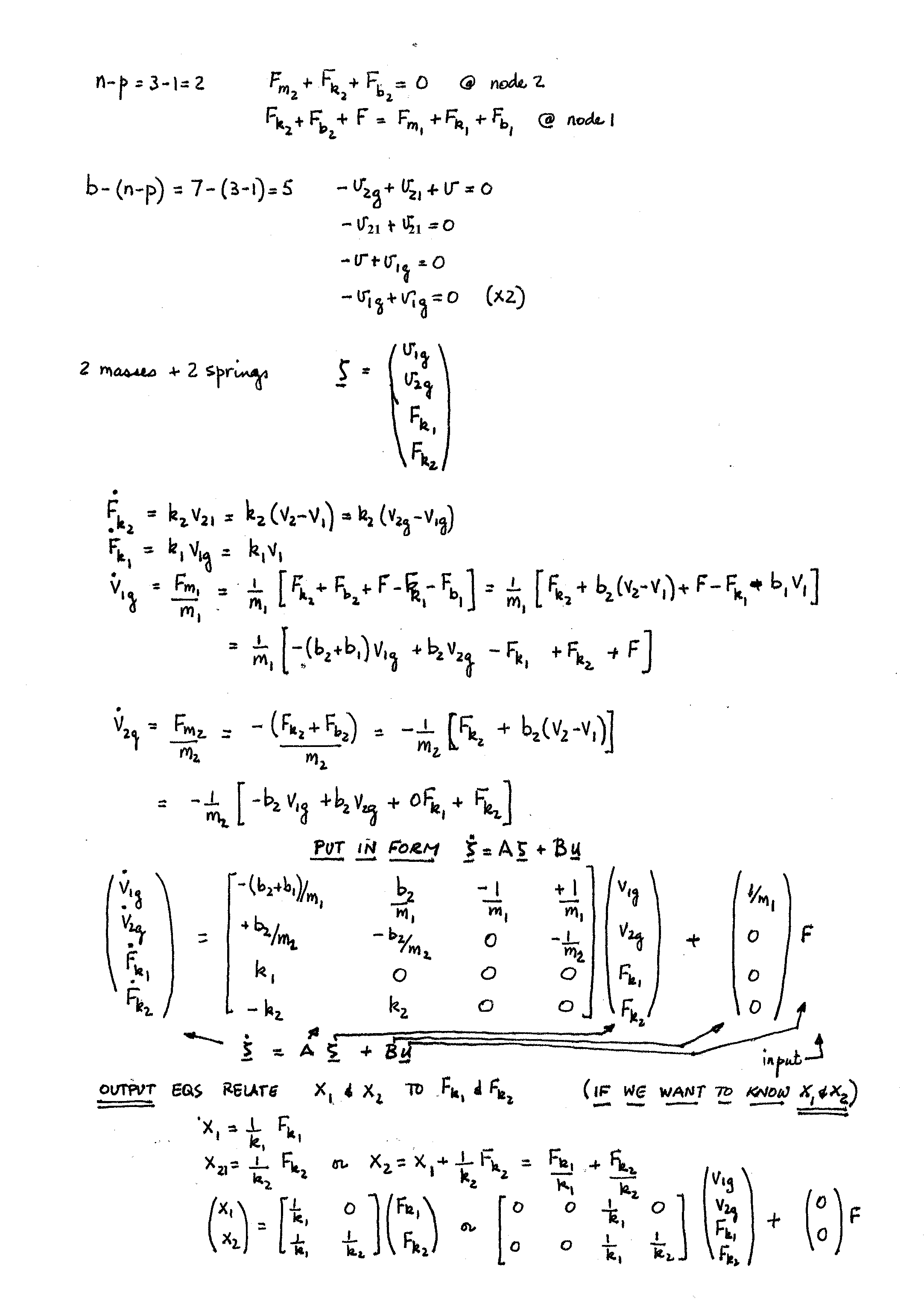
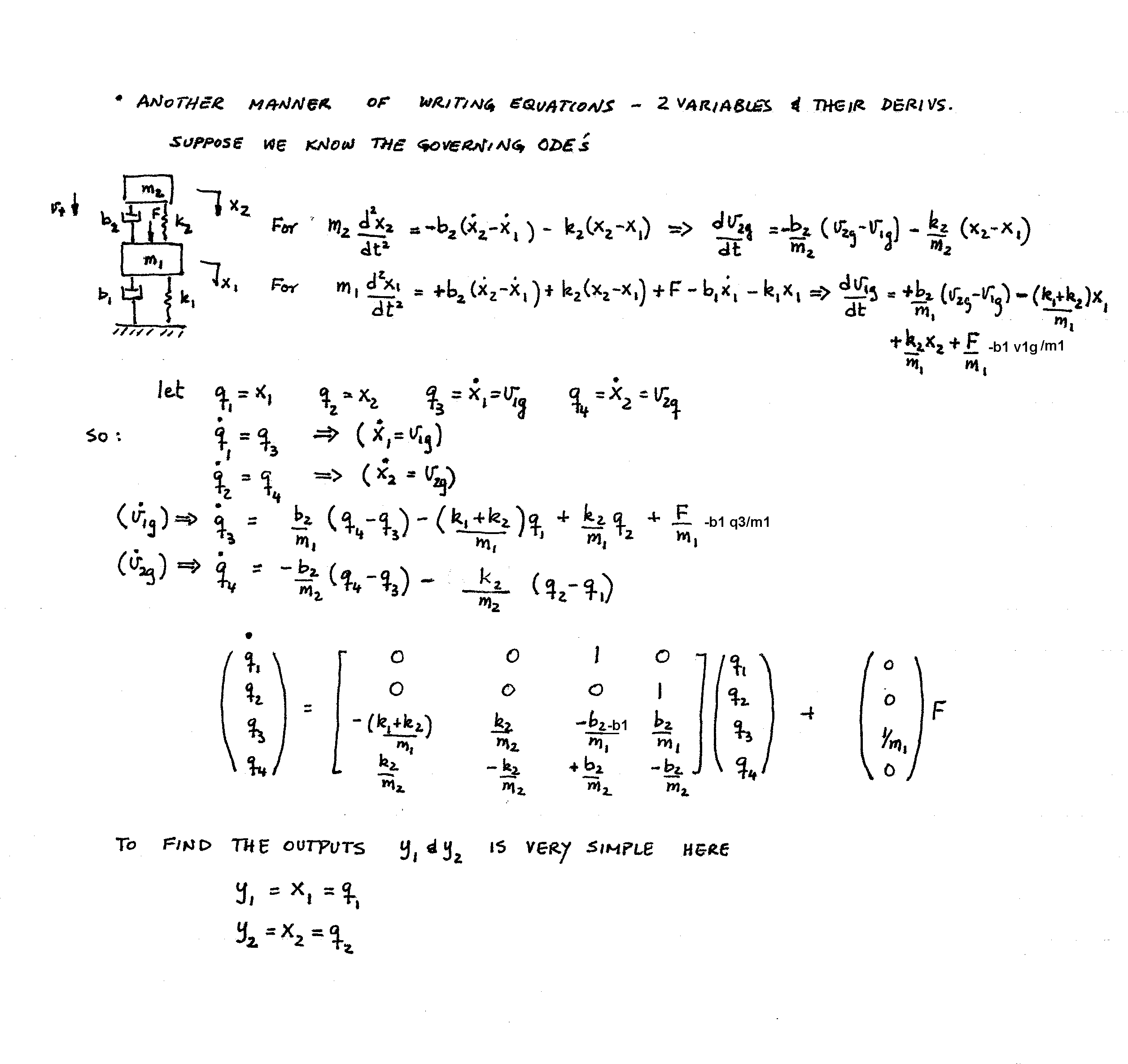
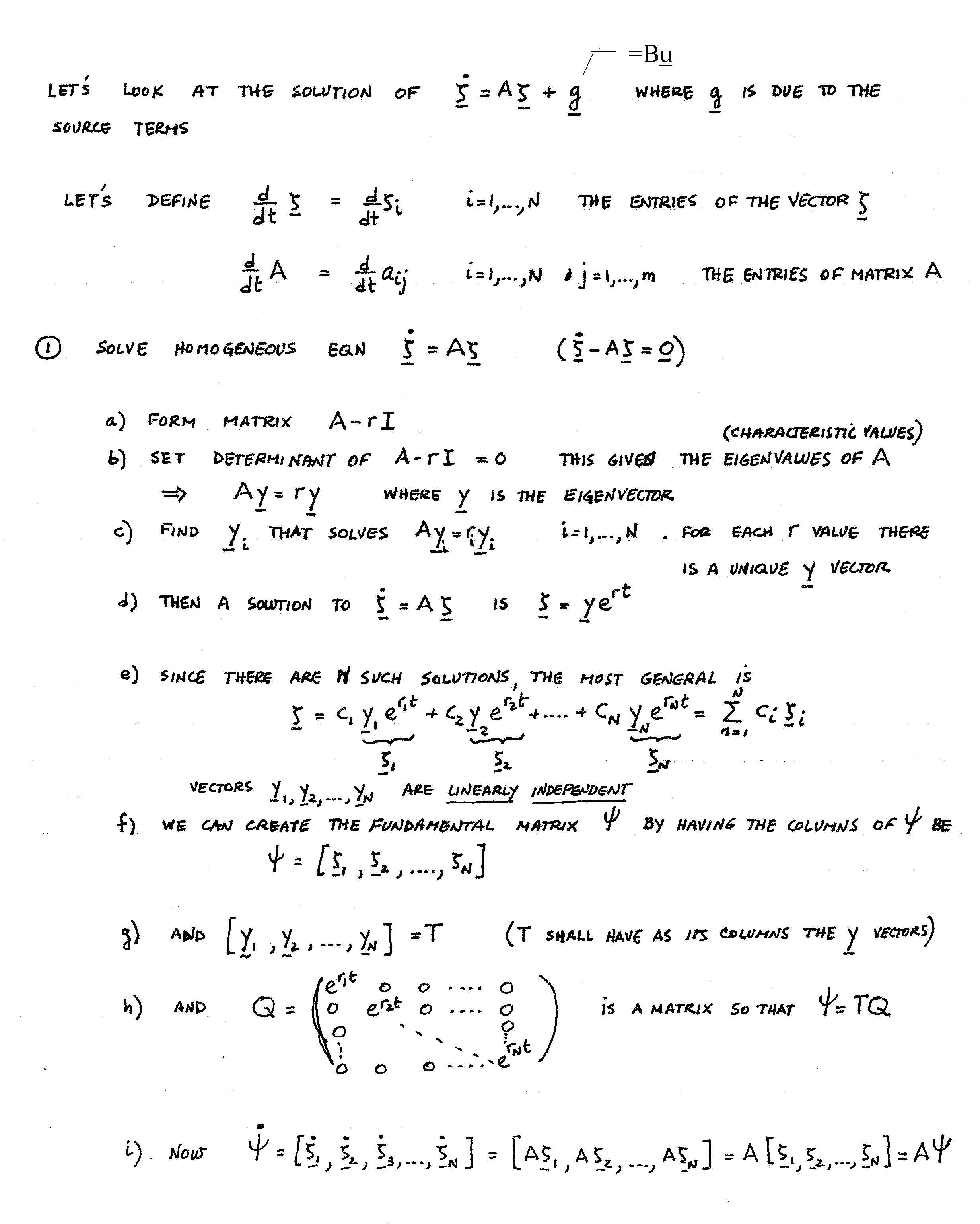
We now begin talking about state equations.

I AM INCLUDING HERE TWO PDF FILES THAT MIGHT HELP YOU: ONE IS ON LINEAR GRAPHS AND ONE IS ON STATE EQUATIONS. THESE DOCUMENTS ARE THE PRECURSOR DOCUMENTS THAT LED TO THE BOOK SYSTEM DYNAMICS, AN INTRODUCTION, BY ROWELL AND WORMLEY.

Here is the material that goes with Lecture 21 10/10 video: page 54, These are the solution to page 54 top and bottom problems page 55, page 56. We also covered page 57, page 58,

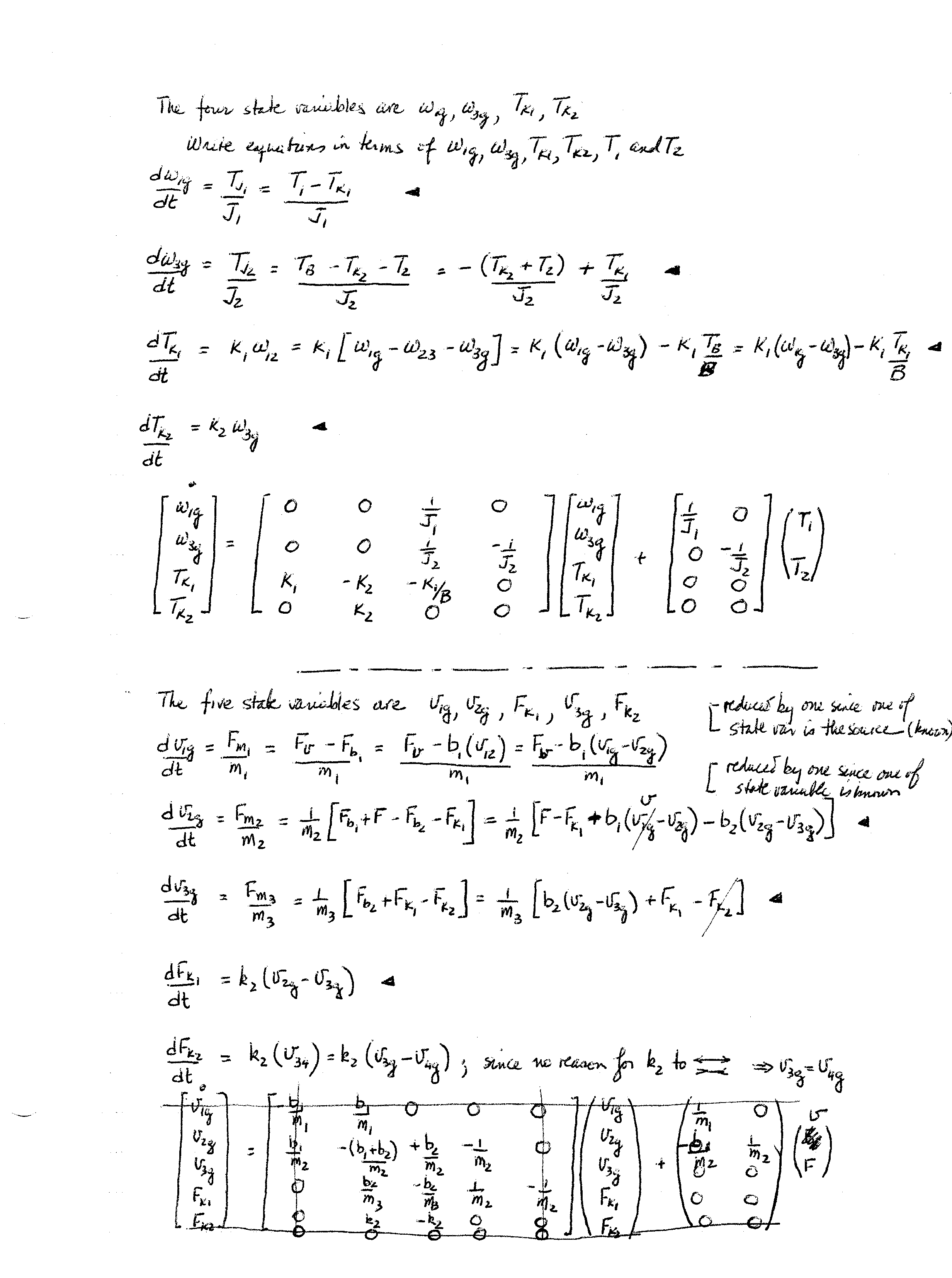
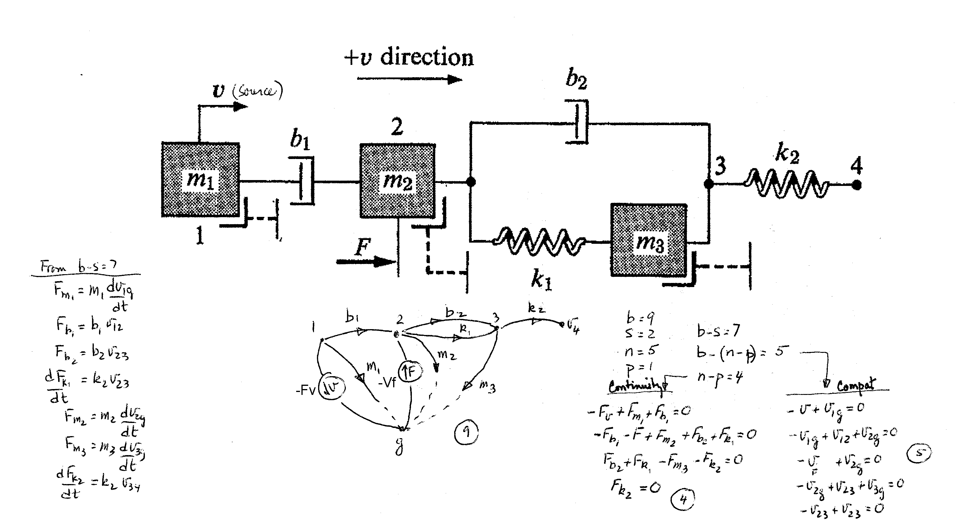
Also look at the STATE EQUATIONS FILE which comes from your book to find more examples for deriving state equations. Please note that the figure numbers used in the file can be found at the end of the file.

You are also suggested to develop the state equations for three problems -- the two problems we did (given on page 54, 55 and 56 of the notes on the website) and problem 6.15 in your book.

We now begin talking about state equation solutions. This solution methodology depends on understanding matrices. For those who need a review of matrices, here it is.

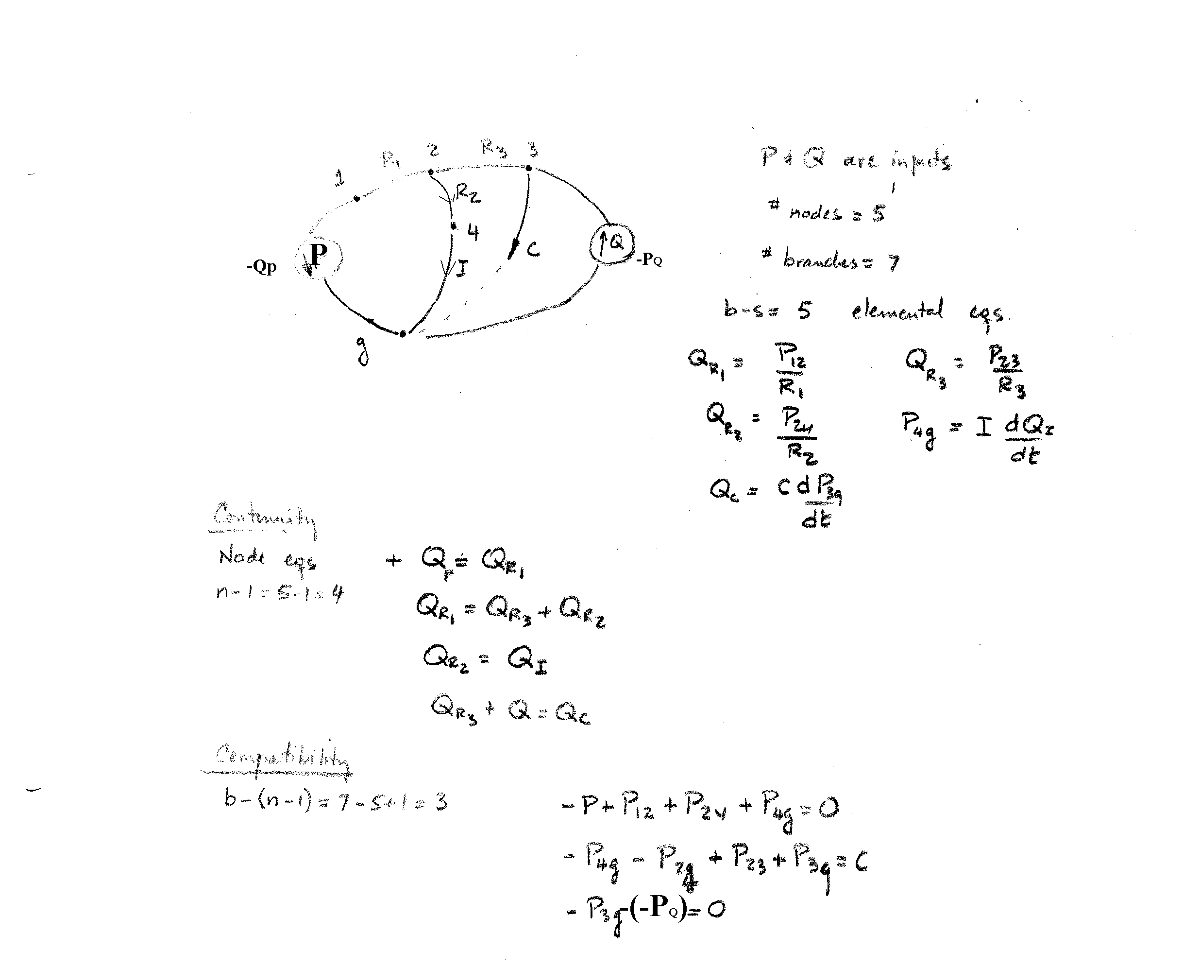
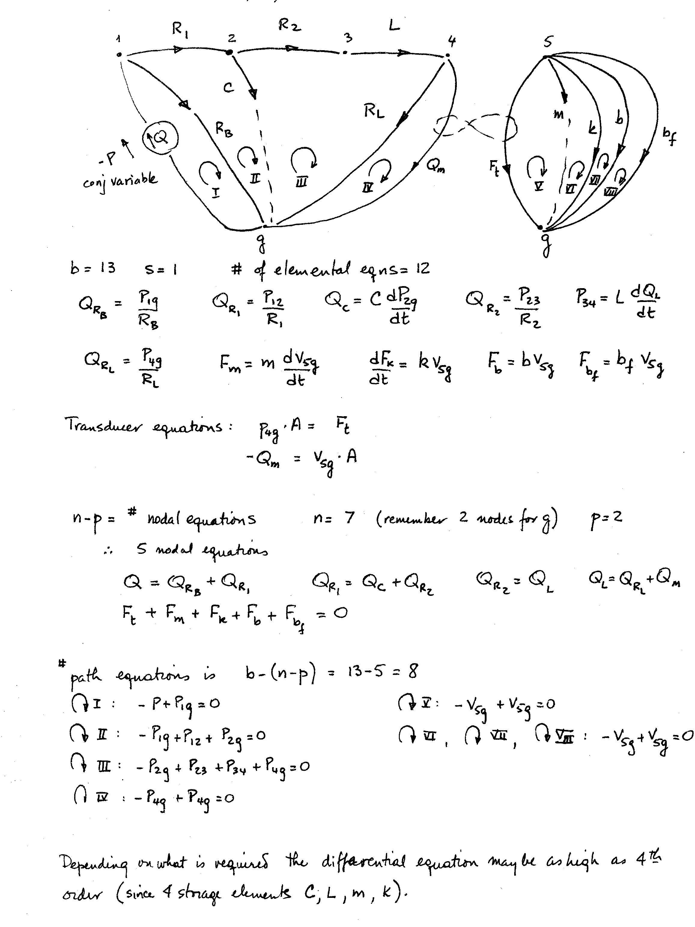
Here is the material that goes with Lecture 22 10/13 video: discussed state variables and how to get the state variable equations and how to solve state variable equations- page 57, page 58, page 59, page 60, page 61, page 62, page 63

As a way of understanding what was covered in today’s class, do the following problems:

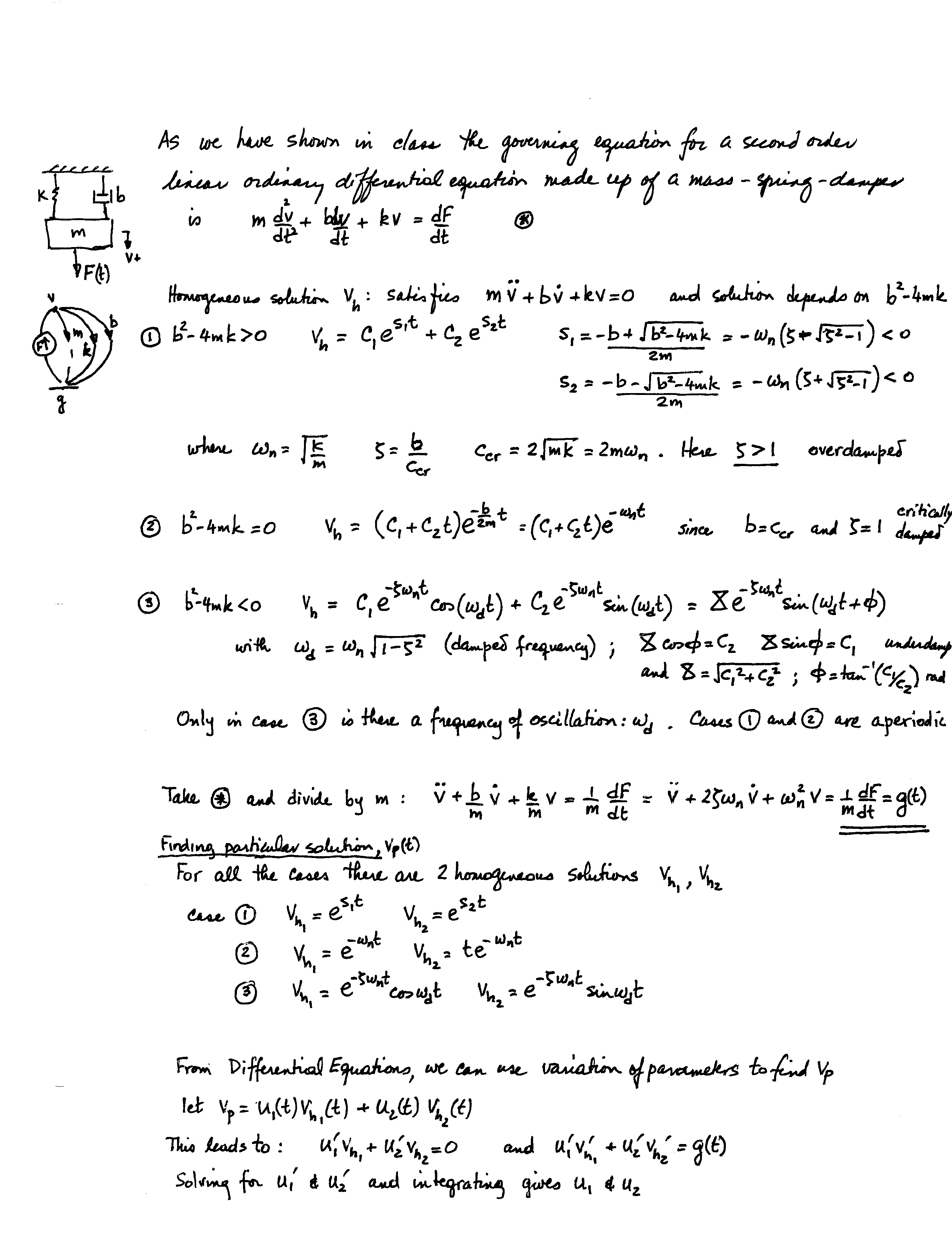
Solve these and and

The solution to these problems will be revealed at the end of the week.

Next exam is announced for November 4 (please note change): materials related to getting system graphs; elemental, vertex, loop equations will be on exam. Further announcements will be made closer to the exam date.

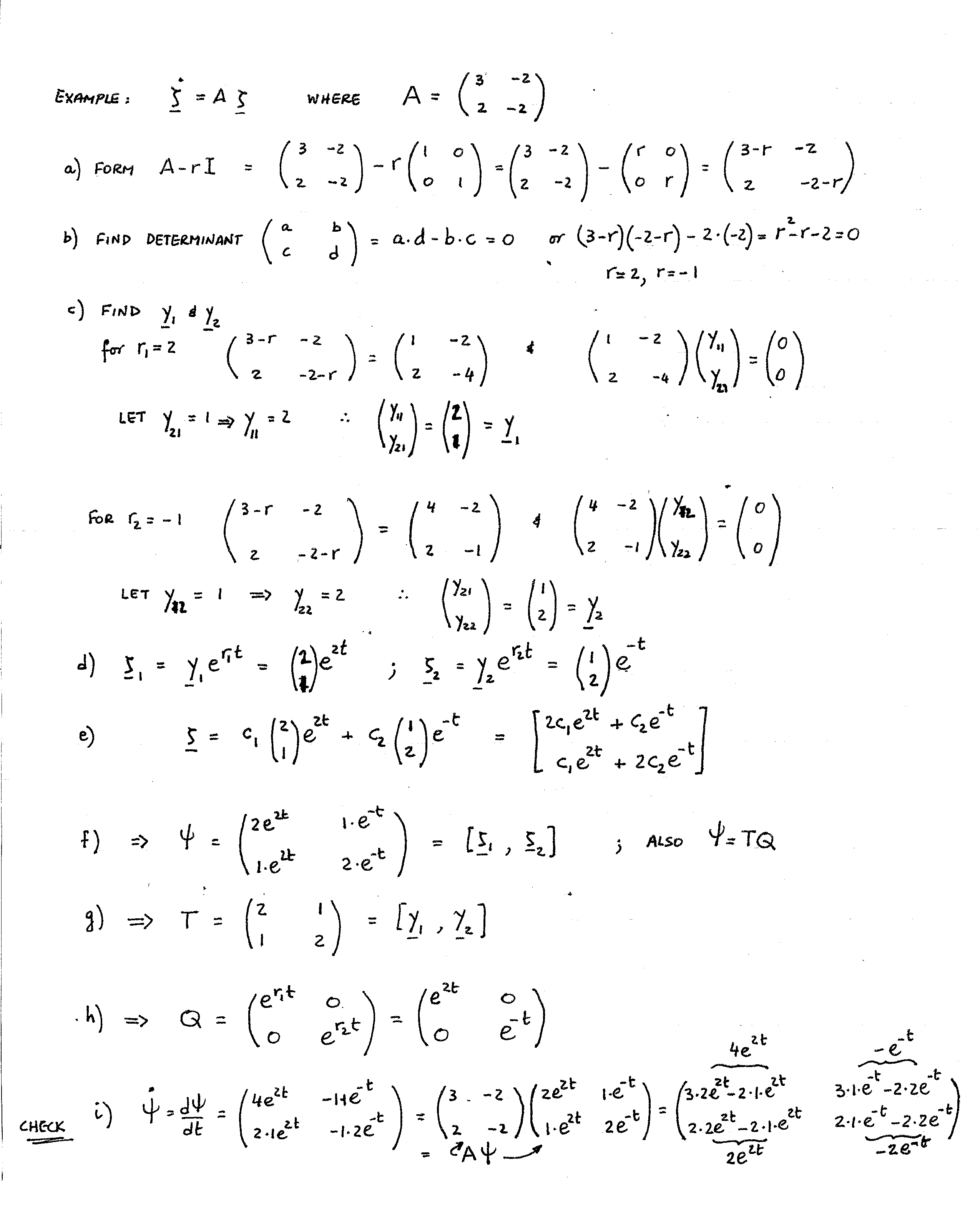
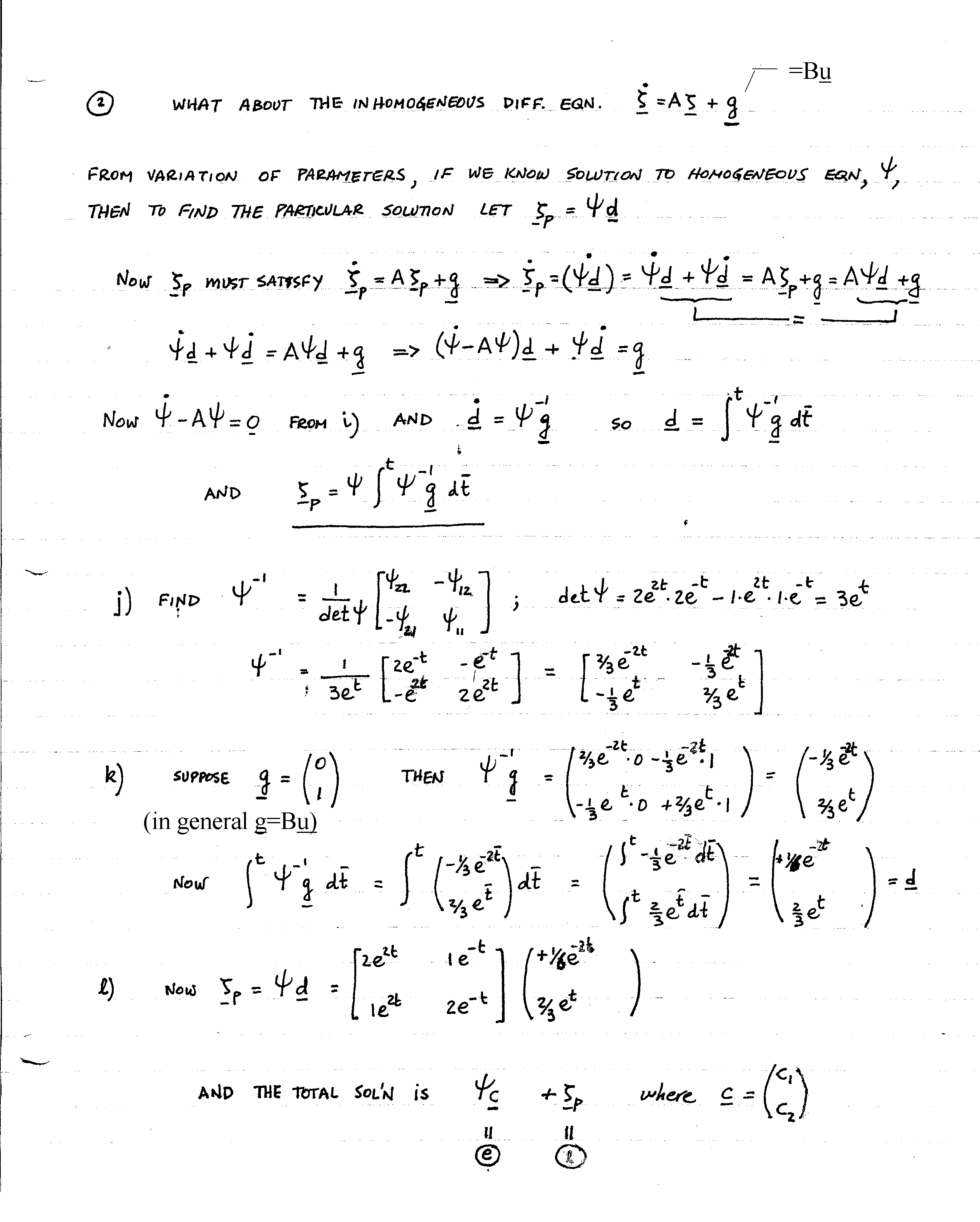
Here is the material that goes with Lecture 23 10/17 video: We reviewed finding the particular solution and how to deal with equal roots page 63, page 64 Another example for you to review on solution of matrix differential equation for the following matrix problem

One of the students asked about how to handle the situation where the A-lI=0 leads to complex eigenvalues. Here is a document that gives an example of what to do.

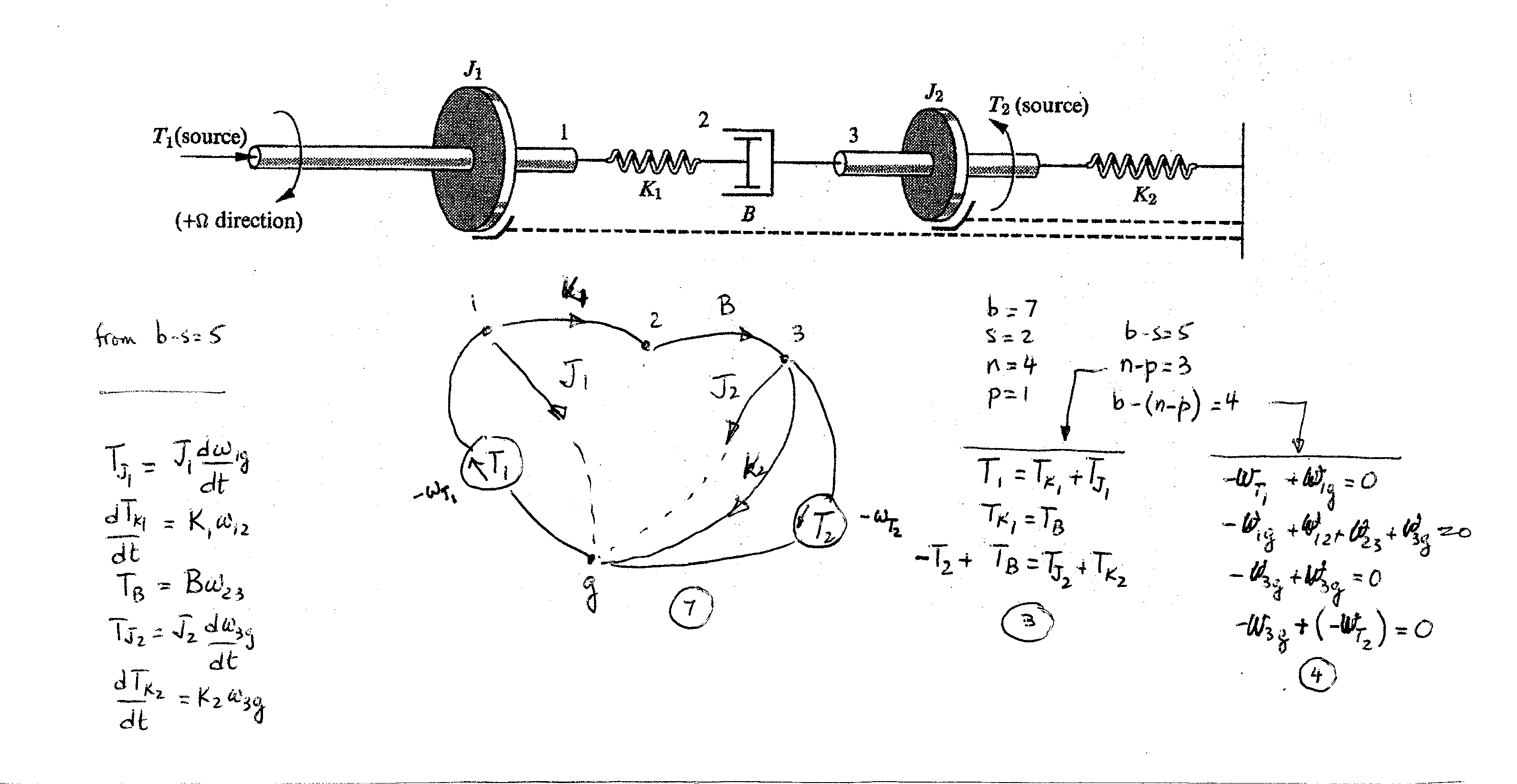
As a review of system graph and state equation derivations look at this problem. The state equation solution is given in the top half of the page.

Here is the material that goes with Lecture 24 video which is the second half of the lecture for 10/17: The following system is discussed including getting the system graph. We also show the state equation solution which is given in the bottom half of the page.

Exam November 4 (please note change): In addition to the two pages you had from exam 1, you can add 3 more 8.5 x 11 formula sheets for the second exam. materials related to getting system graphs; elemental, vertex, loop equations.

We discuss numerical solutions of the state equations in Lecture 25 for the 11/7 class. The materials which were discussed at the end of Lecture 24 tape is given for the numerical solution of these state variable equations page 65, page 66, A handout will be given and discussed on 10/24. The handout is from Applied Numerical Methods by James, Wilford and Smith, pages 339-345 and 351-353.

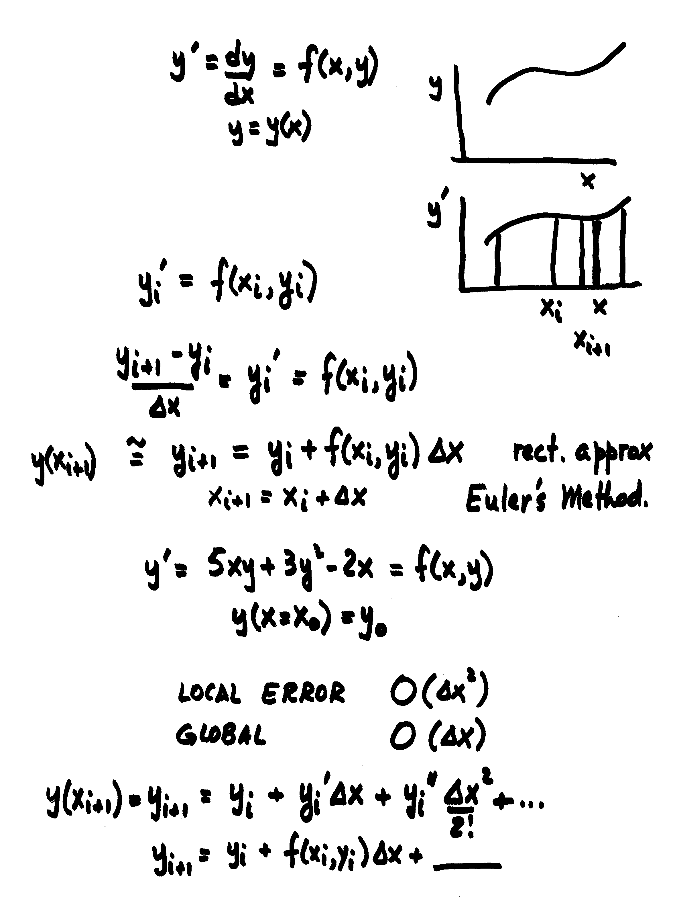
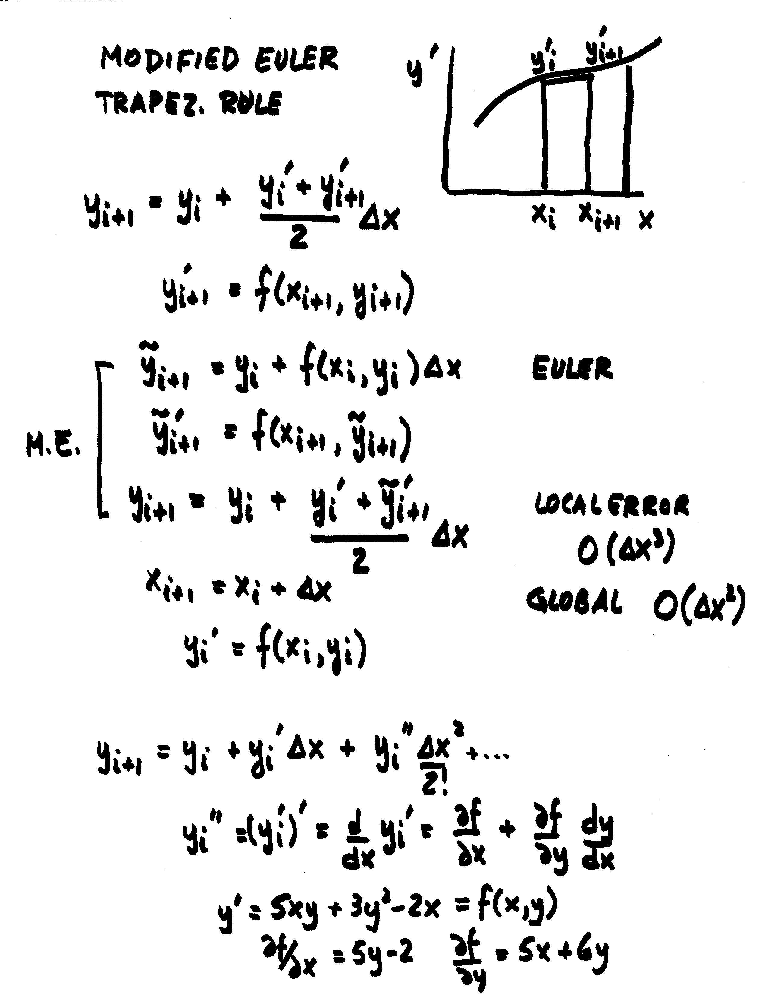
We continue our discussion of numerical solutions of the state equations in Lecture 26. the rest of the numerical solution of sets of first order differential equations was discussed. A handout was given in class on the Runge-Kutta method. The handout is from Applied Numerical Methods by James, Wilford and Smith, pages 339-345 and 351-353. I have copies in my office. If you missed class, stop by my office to get your copy. We plan to look at several examples and how they could be used in the different numerical methods discussed, namely: Euler, Modified Euler, Runge-Kutta Second Order method, Runge-Kutta Fourth Order Method

Here is the solution to the matrix differential equation problems given above– Problem 1 and 2, Problem 3.

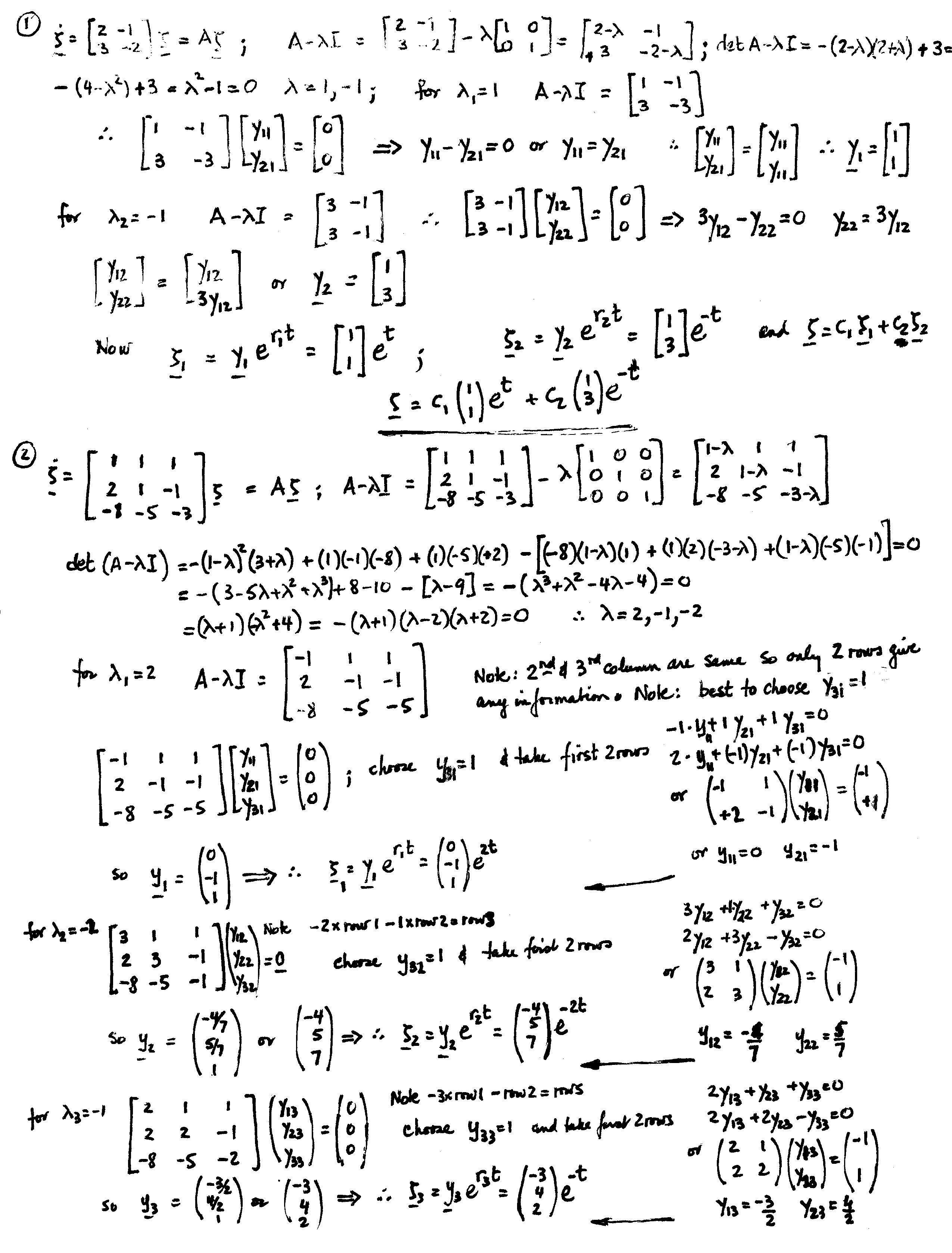
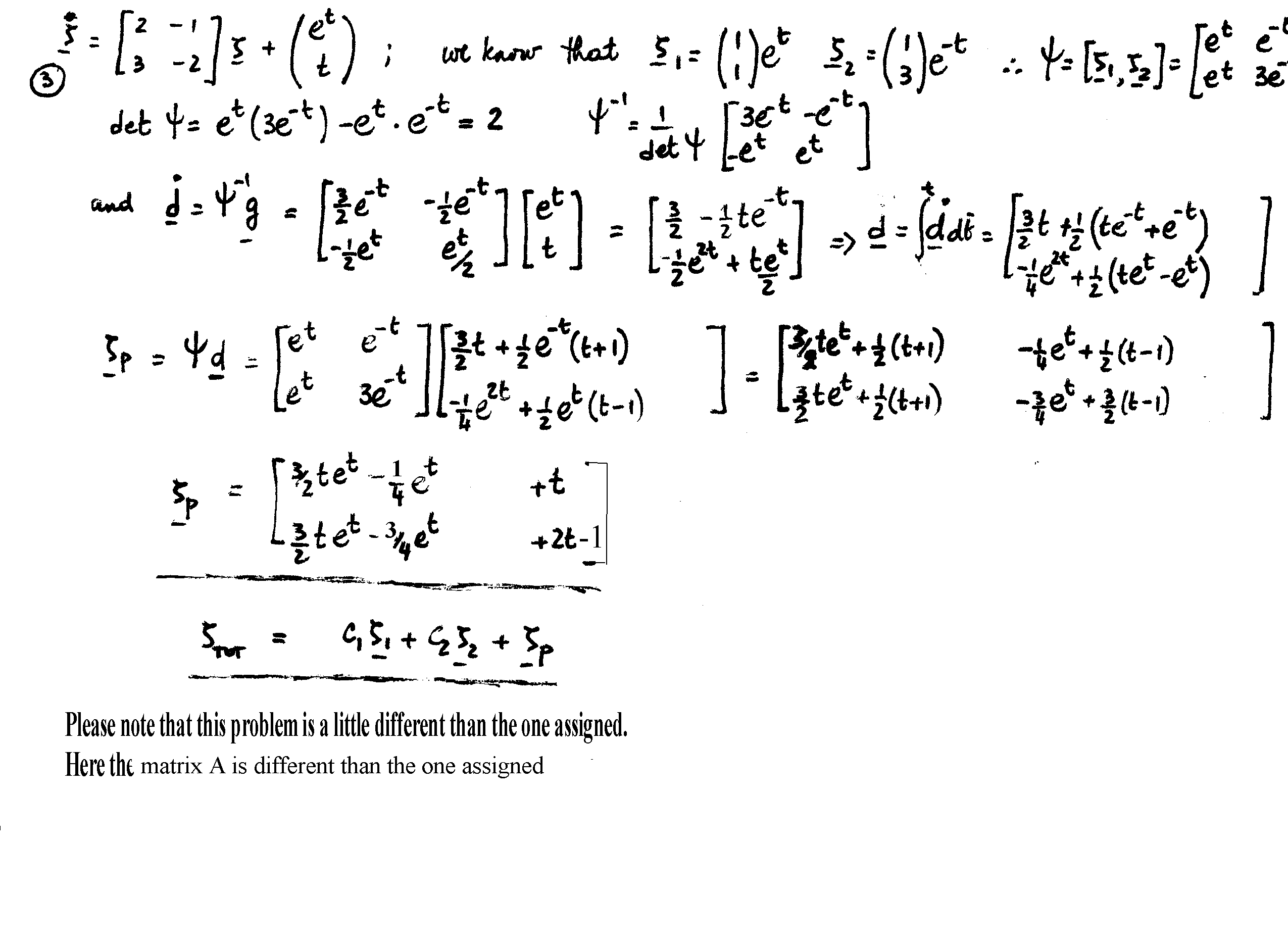
The last exam which will deal with both the analytical solution of matrix equations and numerical solution of differential equations will occur on Nov 28.

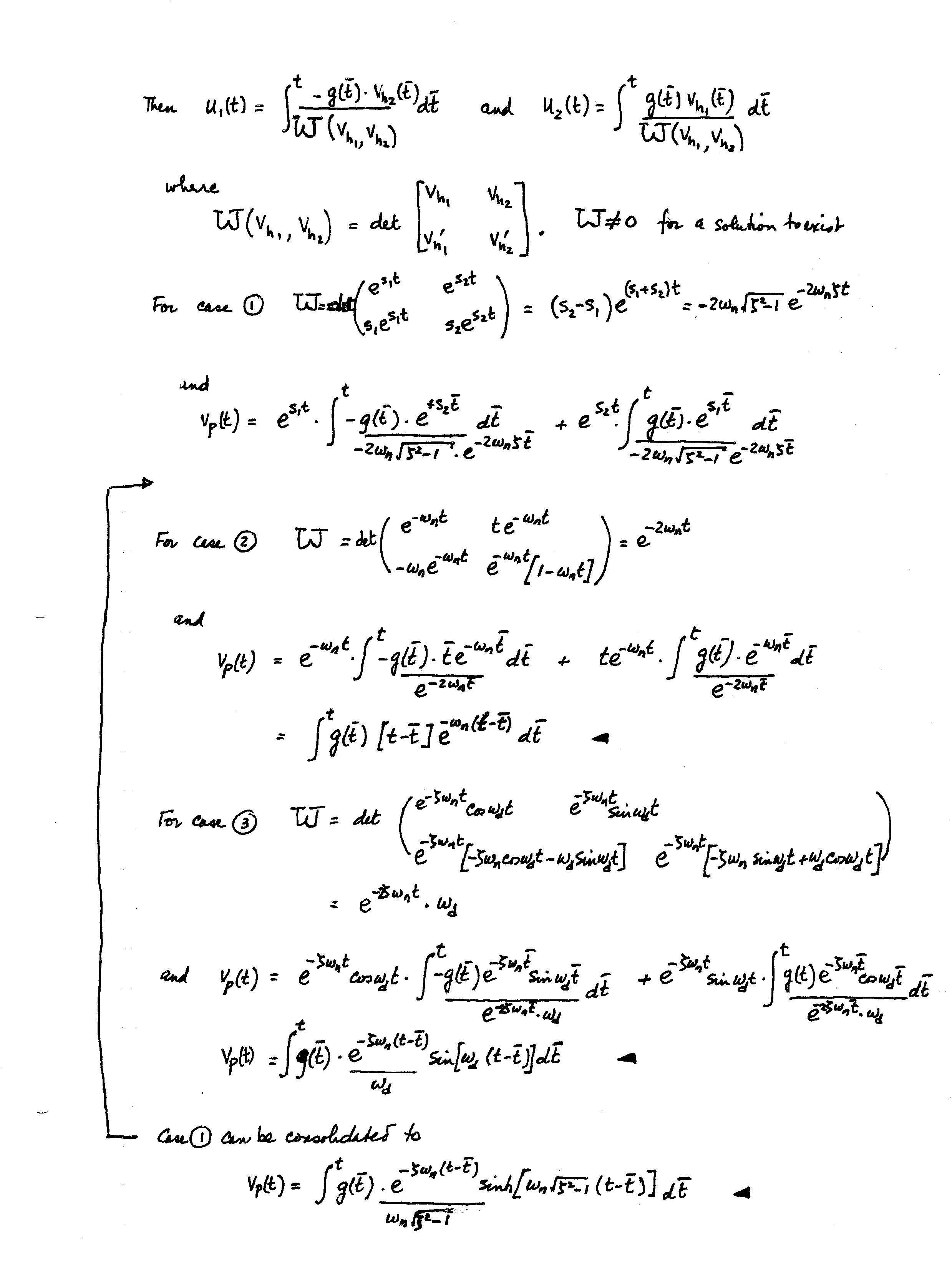
On November 14, we will look at examples related to numerical methods discussed on Nov. 7. We will then move on to solution of inhomogeneous 2^nd order ODEs and inhomogeneous 1^st order ODEs that arise from mass-spring-damper systems or spring-damper systems or mass-spring systems.

In Lecture 27 we will discuss the solution of a mass-spring-damper system with general forcing function.

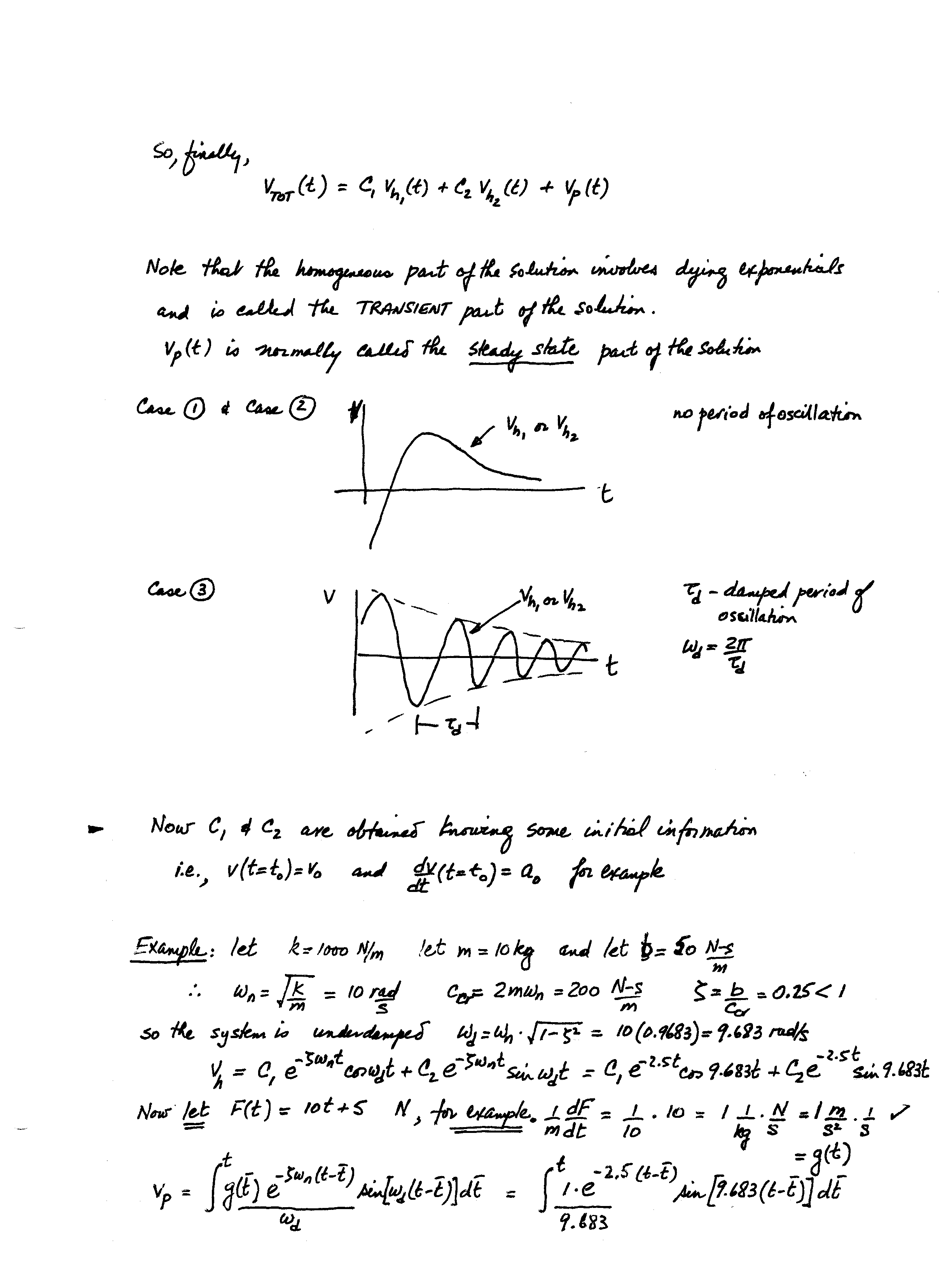
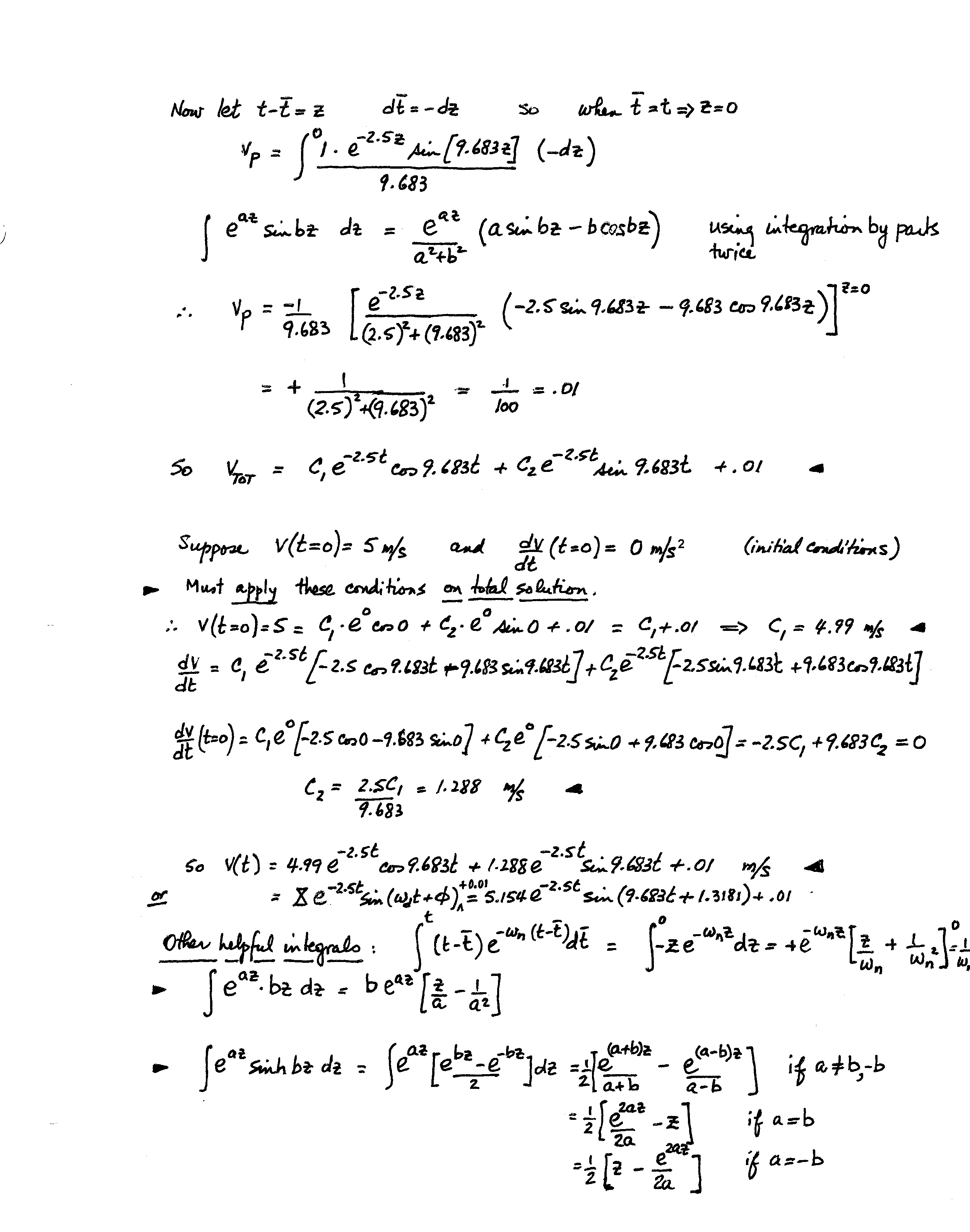
In this lecture covered the solution to the transient and steady state parts of the equation: , which is rewritten as

Please work on problems 8.18, 8.9, 9.8 and 9.23 in your book. The solutions will be revealed on 21 November.

Exam November 28: you are allowed 2 8.5 x 11 formula sheets for the third exam. materials related to solving matrix differential equations and numerical methods will be on exam.

Here are the pages dealing with what we discussed today: page 1, page 2,

Monday 11/28 after the exam we will discuss the following two pages: page 3, page 4.

Here are the solutions to Problem 8.9d in your books and another problem

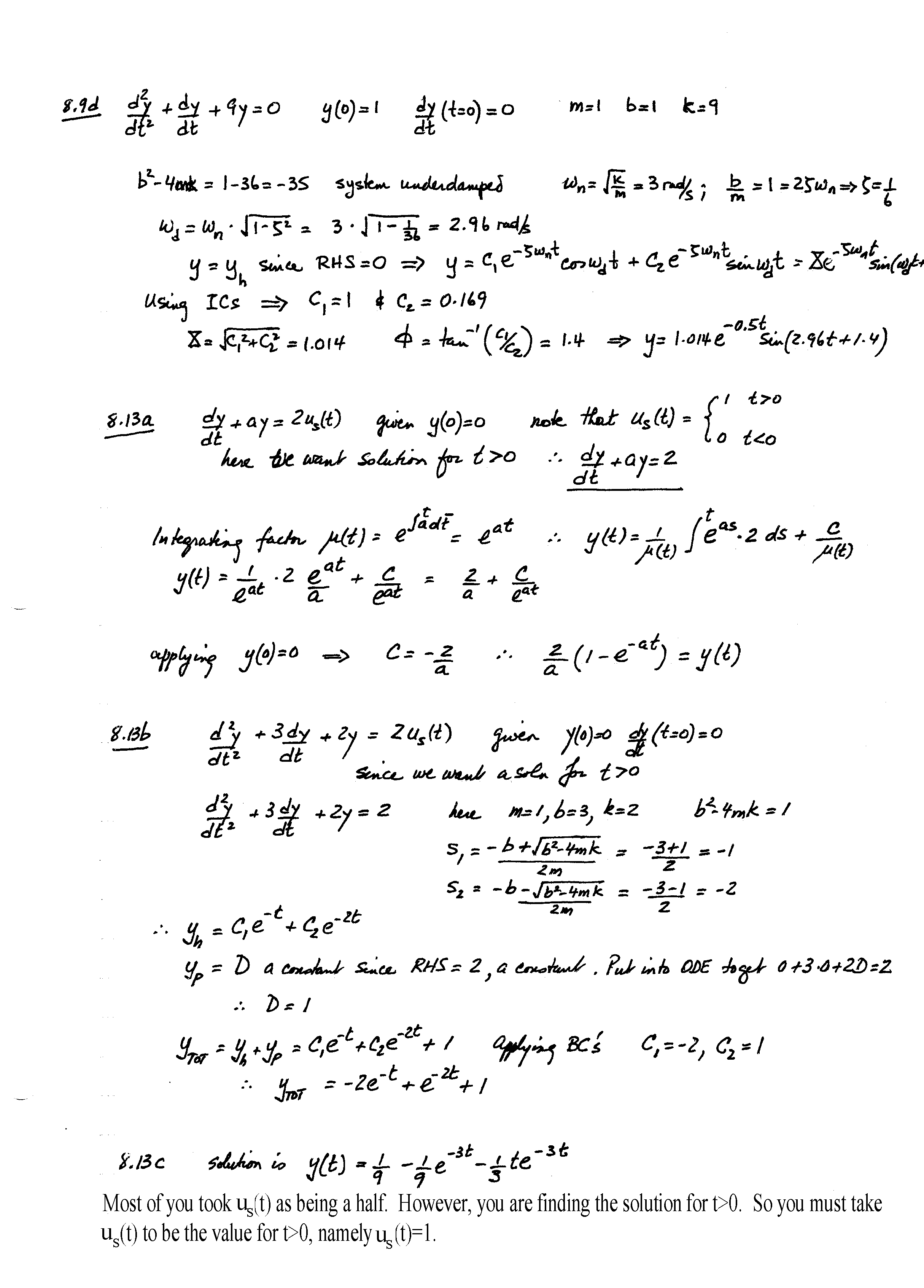
Here are solutions to 8.18 and 9.8

8.18a(i): t=1/2 and y=Ce^-2t . Since y goes to zero as t increases, this is stable.

For (ii) t=-1/2 and y=Ce^2t . Since y goes to infinity as t increases, this is unstable

8.18b:

(i) when a < -1/4 the solutions to the characteristic equation are complex. But the real part of the solutions to the characteristic equation is negative, so the behavior is dying oscillatory. Therefore the solution is asymptotically stable in that the solution goes to zero as t increases, but it oscillates while it goes to zero. The system is underdamped.

(ii) When a=-1/4, the system is critically damped; both solutions are dying exponentials and so the solution to the ODE is stable.

(iii) When -1/4 < a < 0 both solutions to the ODE are dying exponentials and the solution is stable. This is an overdamped system since both rooms of the characteristic equation are negative.

(iv) When a=0, the solution to the ODE is unstable; one solution is a dying exponential but the second is t which increases as t increases.

(v) When a > 0, both solutions to the ODE are increasing exponentials; and so the solution to the ODE is unstable.

8.18c: solutions are sinusoidal and so the solution is neutrally stable as they oscillate about the y=0 line.

9.8 has no state variable since the velocity of the mass, v, is the same as the source, which is assumed known for all time.

But, the governing equation is (m/B) dv/dt + v = F_v(t)/B where -F_v(t) is the conjugate variable to the source. Here (m/B) is the time constant of the system. Since v is known for all time and so is its derivative, then the left hand side is known for all time. Thus the conjugate variable can be calculated for all time.

To determine the time constant for a first order equation, make the coefficient of function v =1 in the equation (see previous paragraph), then the coefficient of dv/dt is the time constant.

To determine the time constants (there are two) for the second order system:

Overdamped system: t=1/|s₁| and 1/|s₂|

Critically damped system: t=1/ω_n

Underdamped system: t=1/ζω_n

REMINDER Final exam will be on December 8 in EC1115 between 215-445pm. It is a comprehensive exam that includes the vibrations covered at the beginning of class and the system dynamics. You will be allowed to bring in 7 8.5 x 11 in sheets into the examination:

These sheets should be formula sheets only. Any sheets containing former exams of yours or others will be confiscated and you will forfeit the examination.

It is suggested that your 7 sheets contain

1 sheet on the elemental equations; 1 sheet with the transformer/transducer equations,

2 sheets on vibration related information; 2 sheet related to matrix/numerical methods

Please make sure you take care of your restroom needs before you start the exam. There will be NO bathroom breaks.

Bring a working calculator and backup battery. Turn off all cellphones, iPODs.

Come in and take alternate seats as we do with all exams.

Bring pens, pencils and erasers

I will provide exam and paper.

I will return your last exam on Friday 12/2 so that it will help you get ready for the final exam.

With respect to the sheet that you are allowed to bring into the exam in which you have your numerical methods formulas:

Please make sure you have the information for all the numerical methods we discussed either in class and/or in the numerical methods handout given in class, namely

1) Euler

2) Modified Euler

3) Runge-Kutta 2^nd order which is like the modified Euler

4) Runge-Kutta 2^nd order known as the midpoint method

5) Runge-Kutta 3^rd order

6) Runge-Kutta 4^th order

and how to use these methods if you have more than one state variable equation, as well.

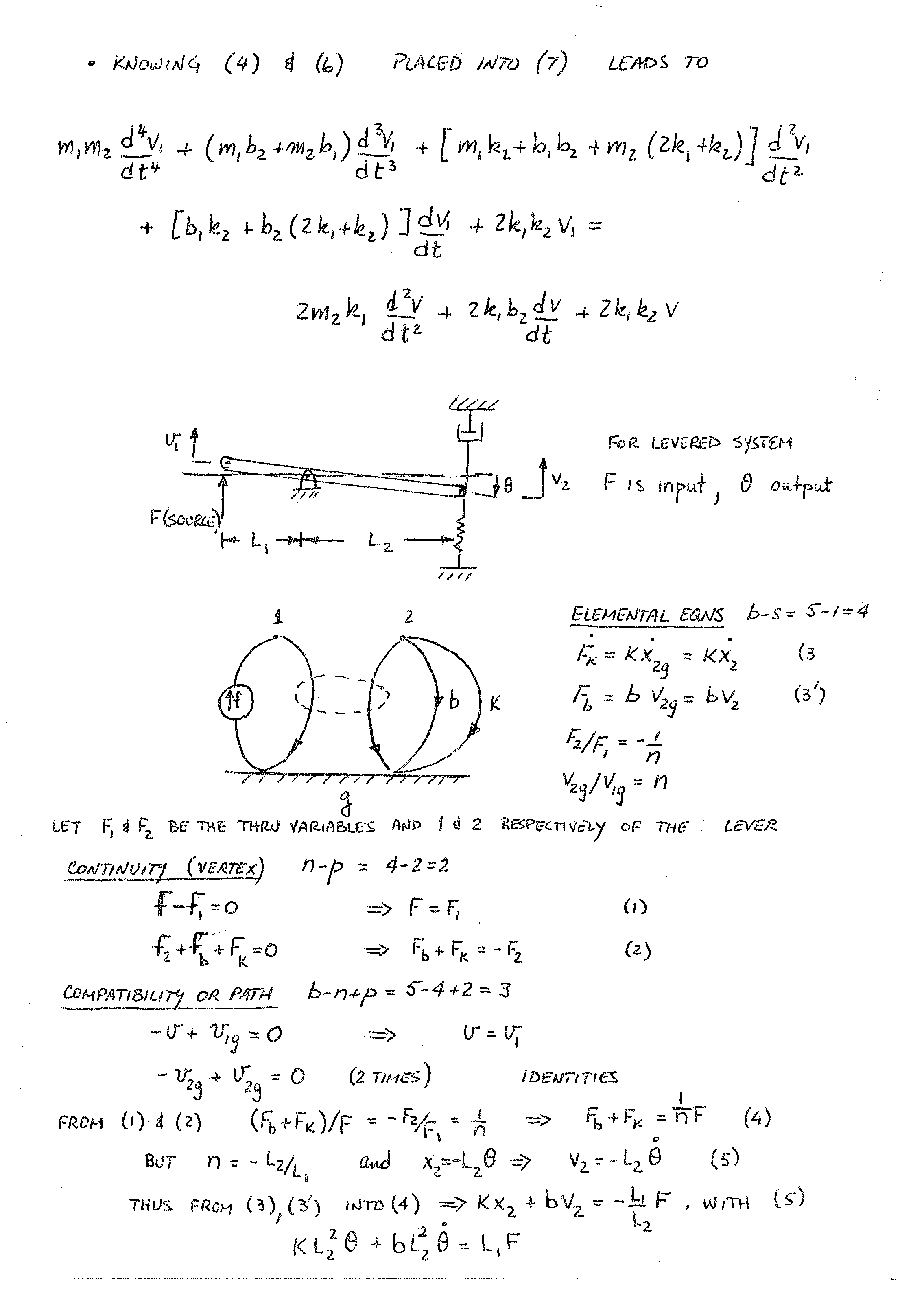
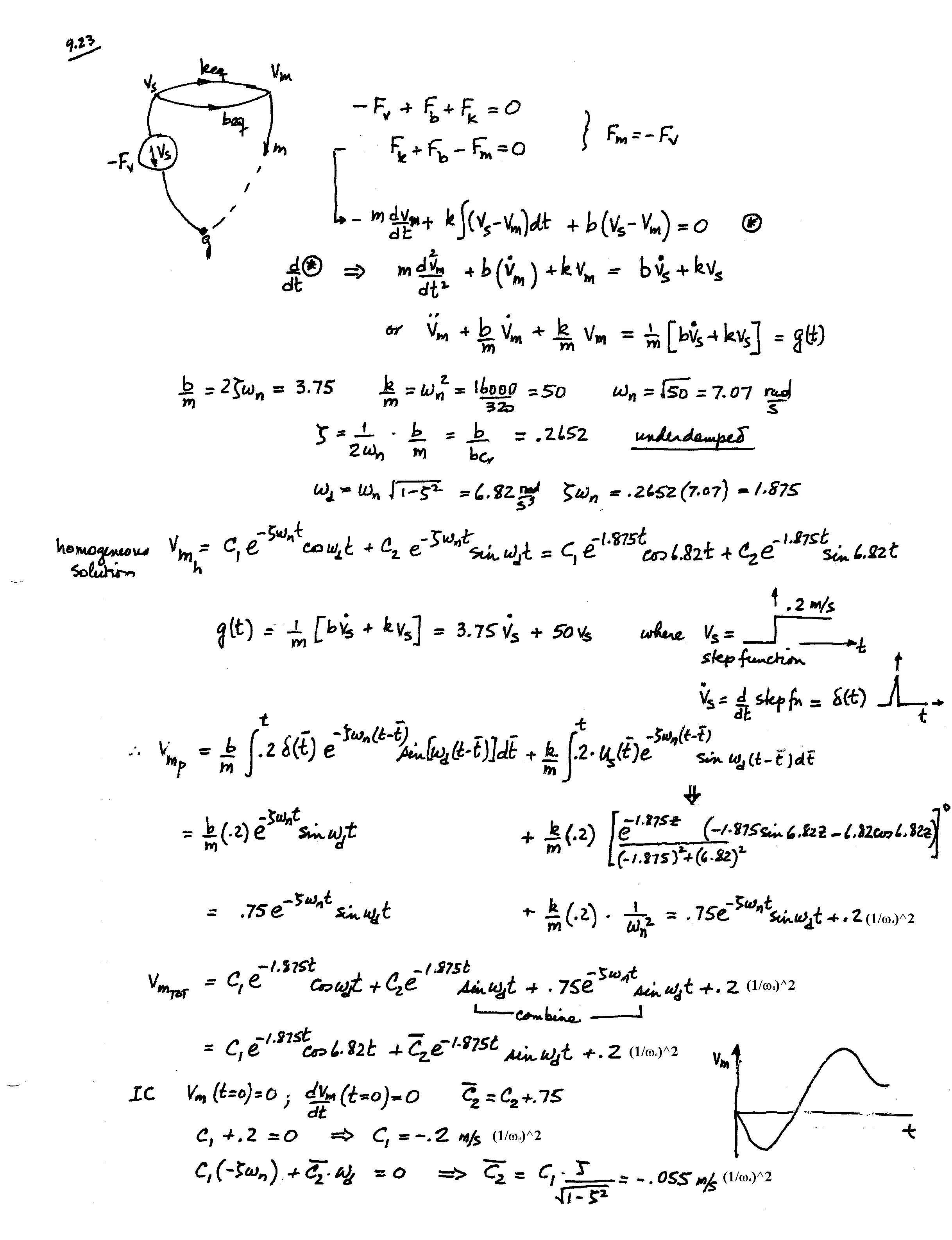
In Lecture 28 we discussed and are discussing the solution of problem 9.23 in your books. Note that the solution is tending towards Vm =0.2 m/s which is the steady state solution of the problem due to the step increase to Vm=0.2 m/s that occurs at t=0+. and here is the solution graph. We also discussed the lever transformer (teeter-totter) when the fulcrum is at rest and when it is acted upon by a source. We discussed the linear graph of the two problems and answered some questions.

We will have a review class on 12/5 between 12-1pm in room EC1112.