EML3222 Fall 2019 page

Department of Mechanical and Materials Engineering

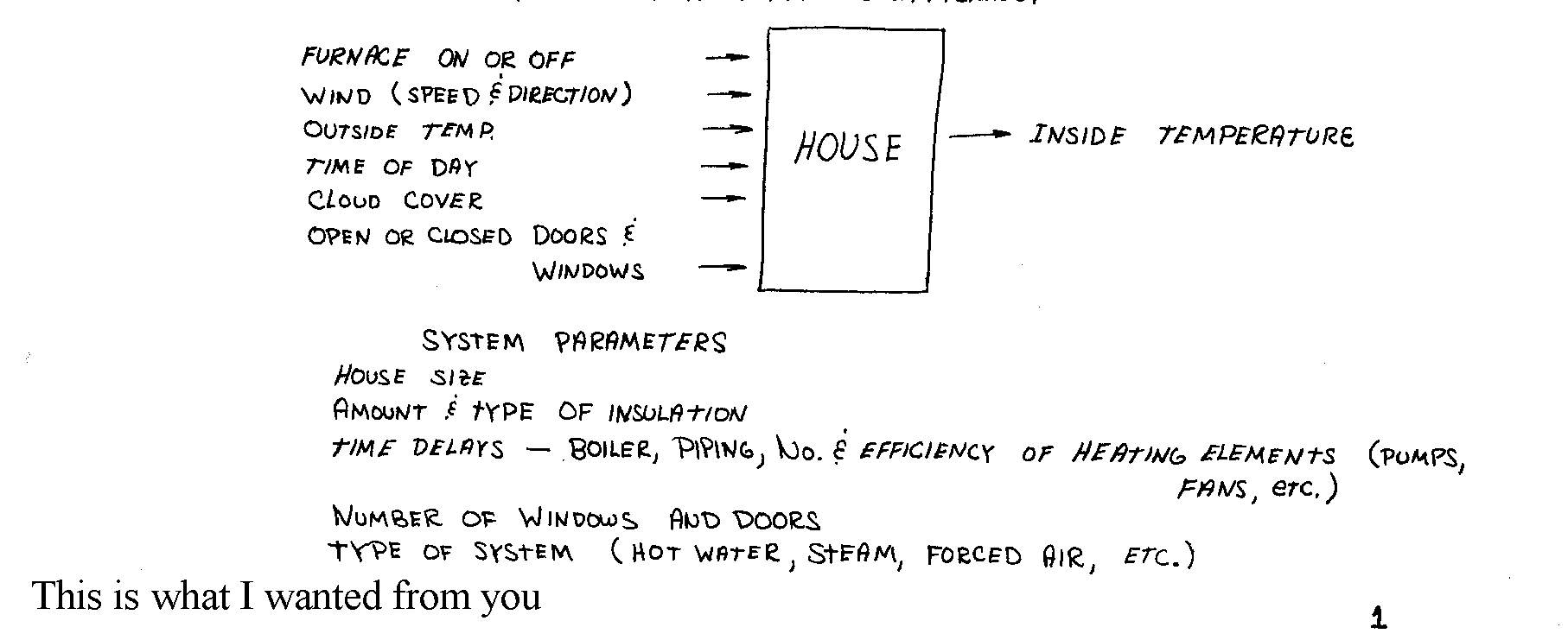
This is Dr. Levy’s EML3222 System Dynamics Fall 2019 page

Florida International University is a community of faculty, staff and students dedicated to generating and imparting knowledge through 1) excellent teaching and research, 2) the rigorous and respectful exchange of ideas, and 3) community service. All students should respect the right of others to have an equitable opportunity to learn and honestly demonstrate the quality of their learning. Therefore, all students are expected to adhere to a standard of academic conduct, which demonstrates respect for themselves, their fellow students, and the educational mission of the University. All students are deemed by the University to understand that if they are found responsible for academic misconduct, they will be subject to the Academic Misconduct procedures and sanctions, as outlined in the Student Handbook.

The FIU Civility Initiative is a collaborative effort by students, faculty, and staff to promote civility as a cornerstone of the FIU Community. We believe that civility is an essential component of the core values of our University. We strive to include civility in our daily actions and look to promote the efforts of others that do the same. Show respect to all people, regardless of differences; always act with integrity, even when no one is watching; be a positive contributing member of the FIU community.

Here is the (08/15/2018) syllabus for the course.

My office is in EC3442, and email address is levyez@fiu.edu

My tel. no. is 305-348-3643. My fax no. is the department fax no. is 348-1932

My Office hours: 230-4pm W; 1230-2pm R; 1030-12pm F; by appointment

TA information: TBD

You will be required to form a group of four students as your study group and also for your project.

This material and all the linked materials provided, except where stated specifically, are copyrighted © Cesar Levy 2019 and is provided to the students of this course only. Use by any other individual without written consent of the author is forbidden.

Photocopies of the 3 material selections relating to vibrations will be available from the department office starting August 20. Please make up your groups of four and one of you come to get the materials. Cost is $15 per set. They will be used in the vibrations section of the course, which will occur later on in the semester. HWs will be assigned from this source later in the semester as well.

Here is Lecture 1 video and here are the pages related to the first lecture: page 1, page2, example, page 3, page 4, page 5

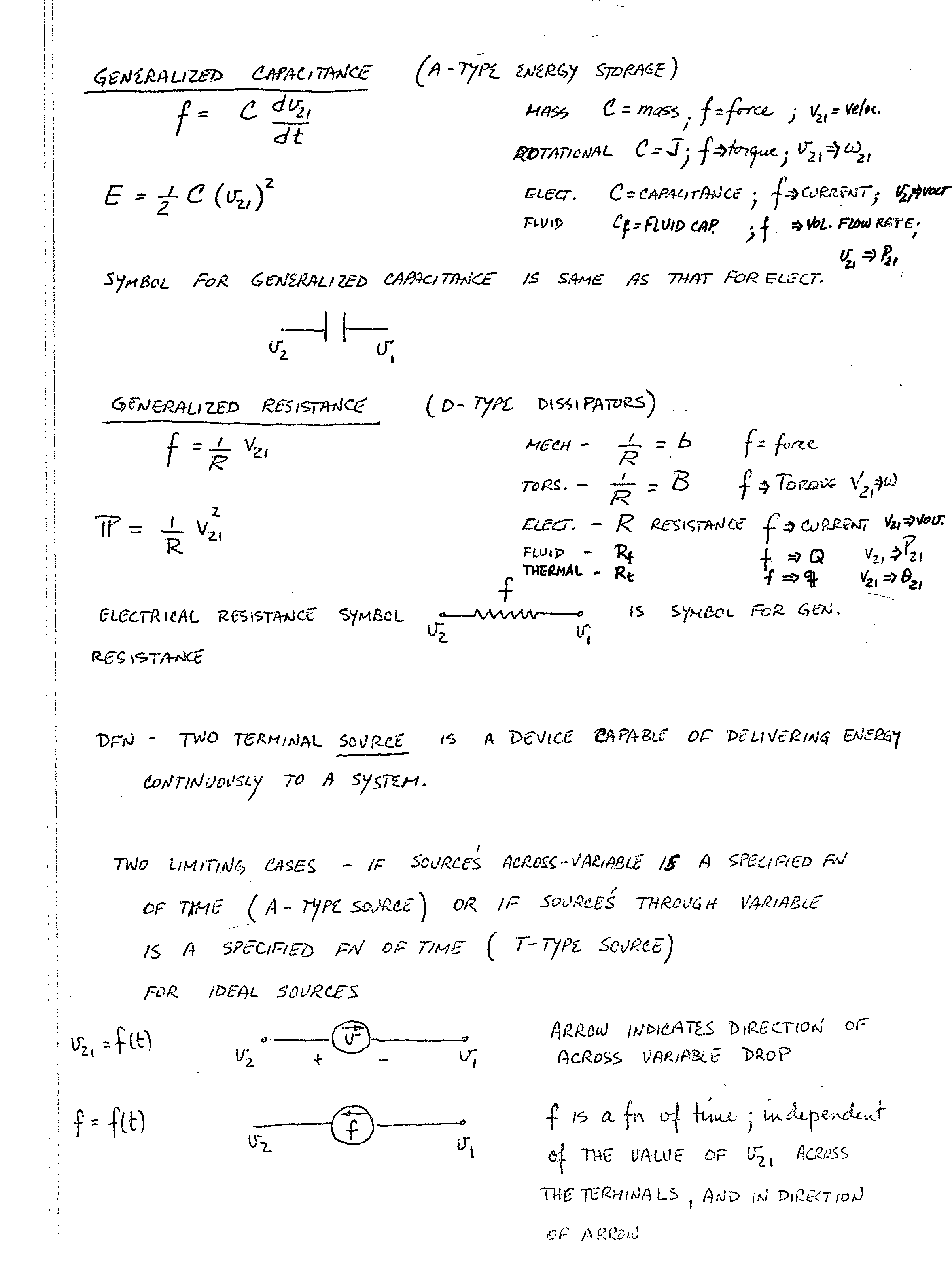
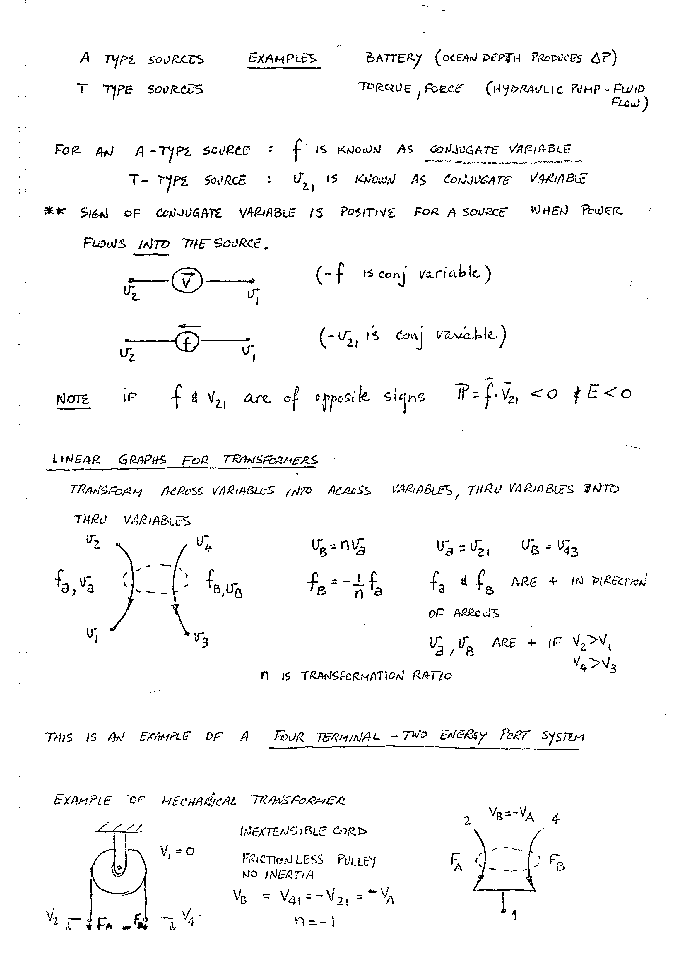
Please read Chapters 1 and 2 of the Rowell and Wormley Intro to System Dynamics book

Here is Lecture 2 video and the pages related to the video: page 6, page 7, and page 8.

Please start reading Chapters 3 and 6 of the Rowell and Wormley System Dynamics book

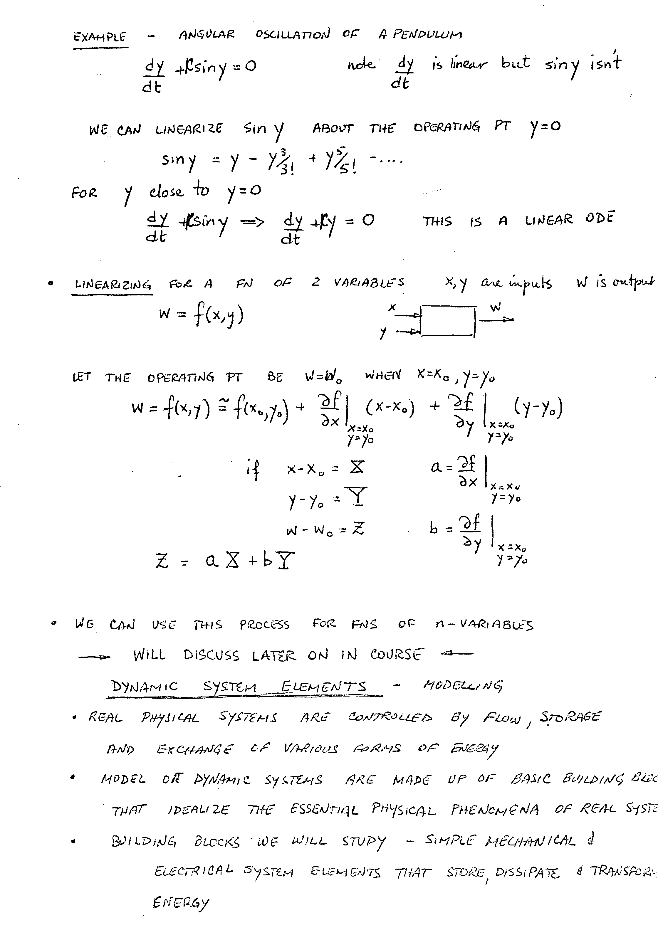
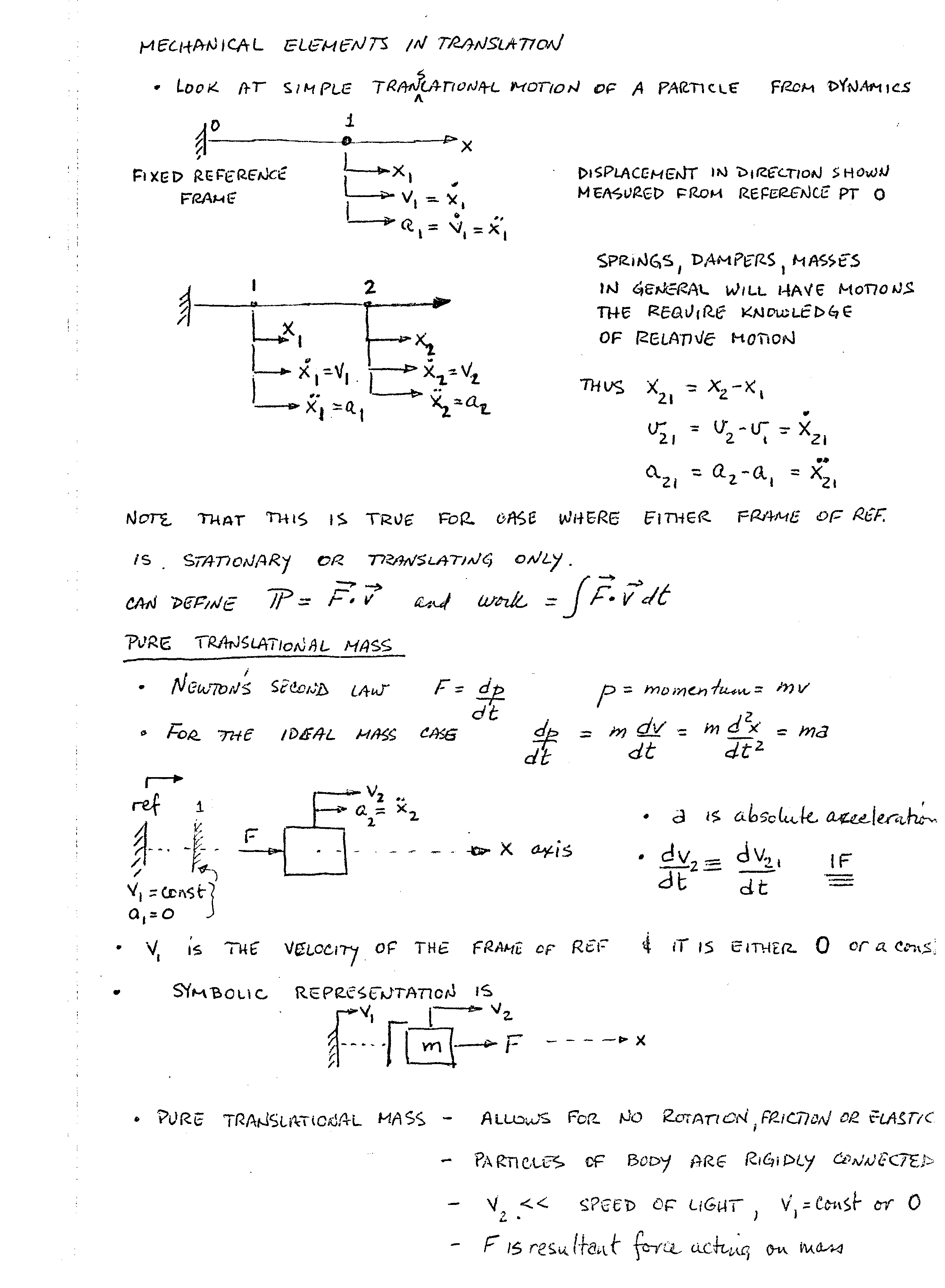
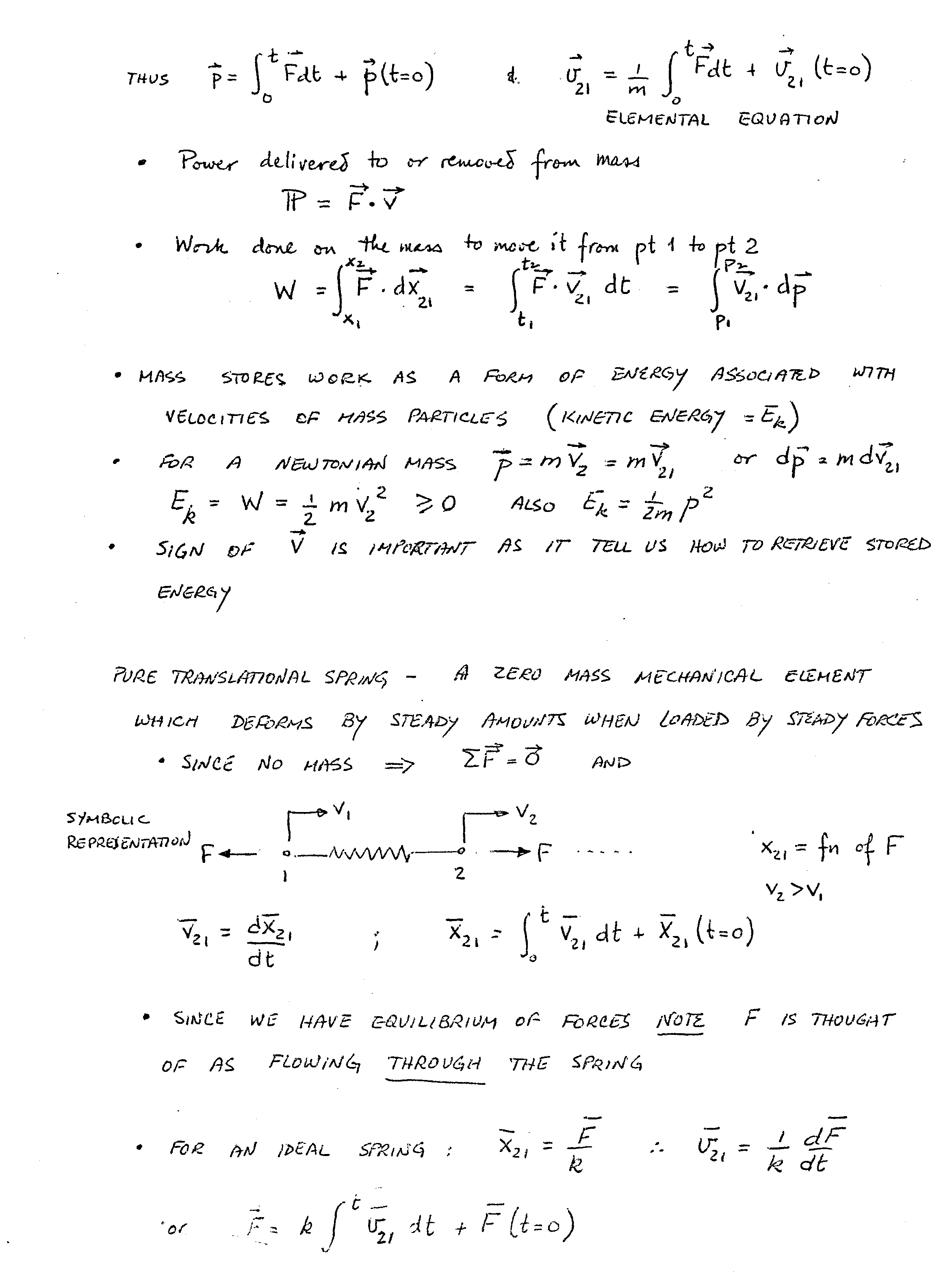
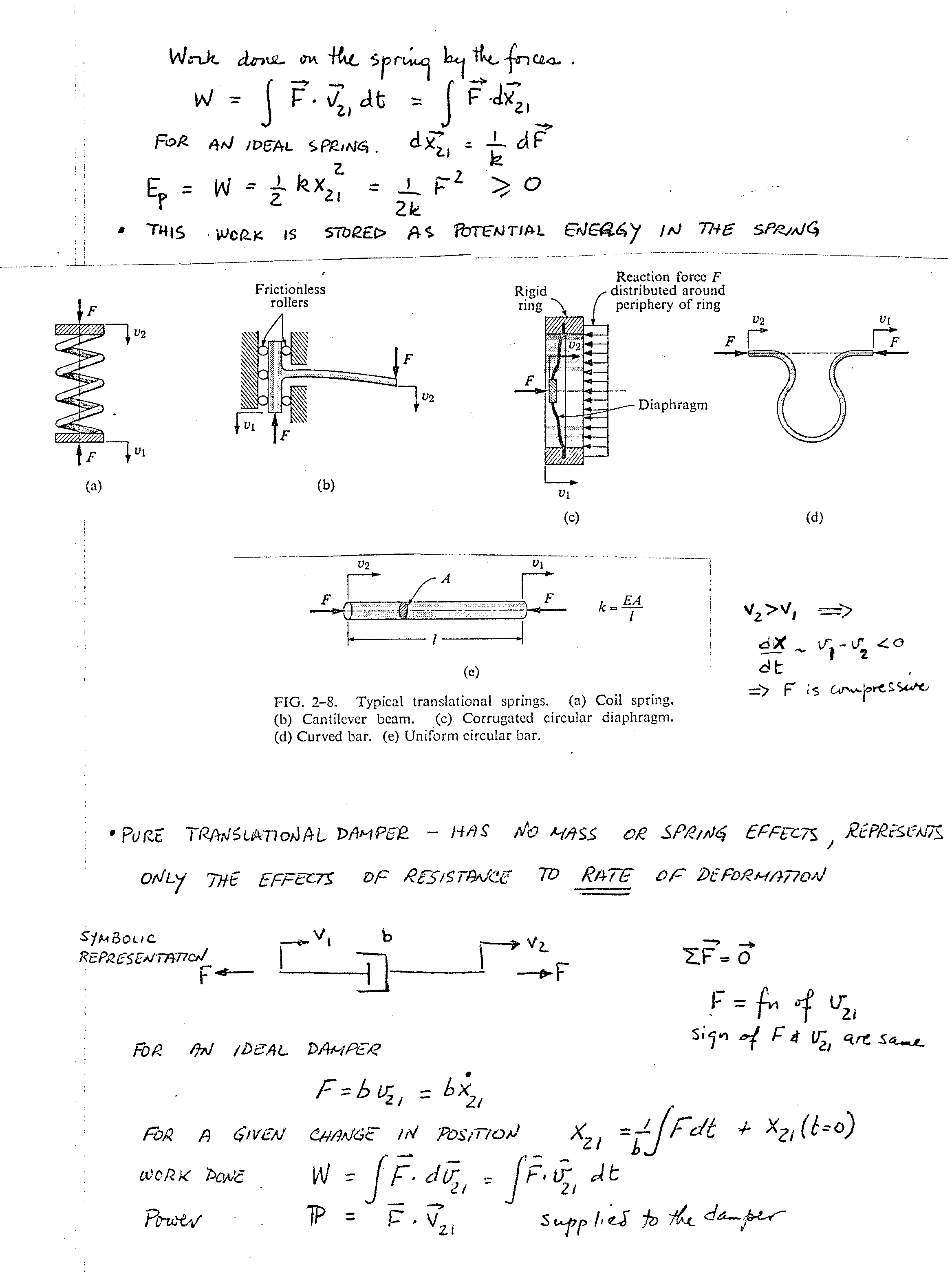
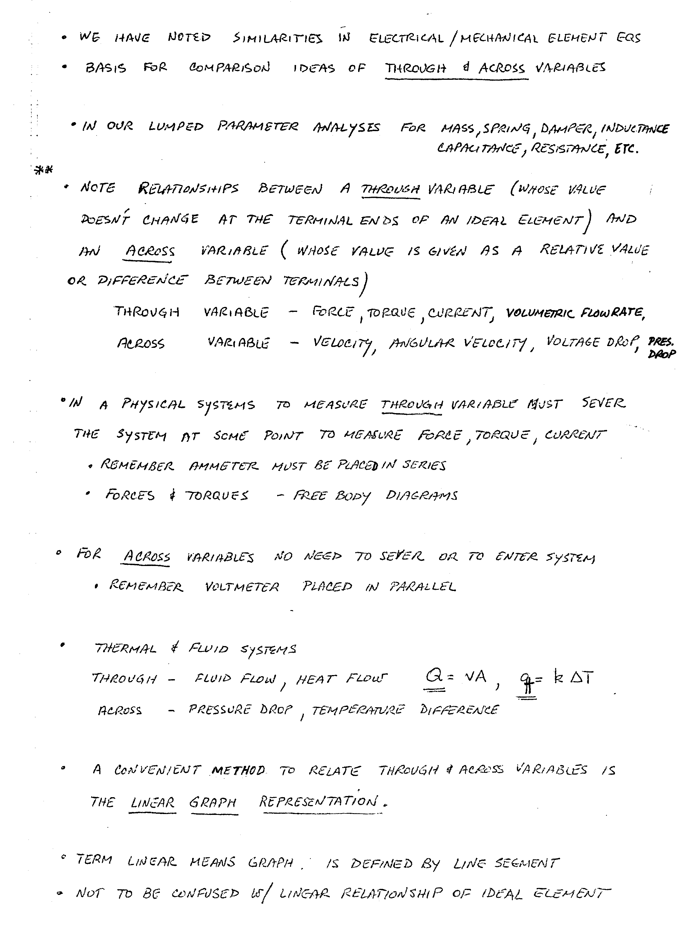
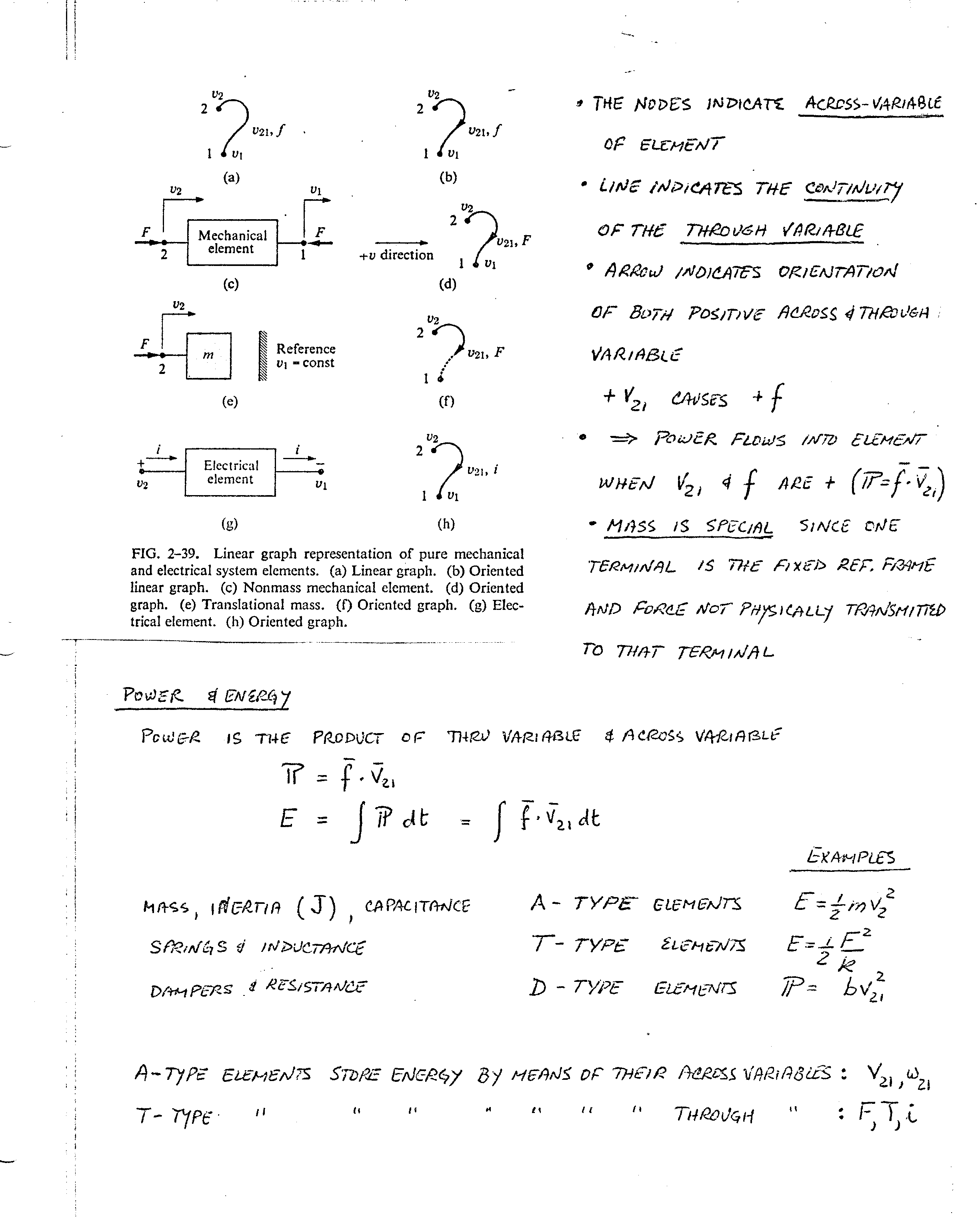
Lecture 3 video: At the 45 minute mark of the video we begin the topic of system dynamics by defining the through and across variables, the elemental and constitutive equations, the ideal and pure element. page 9, page10, page11, examples, page12,

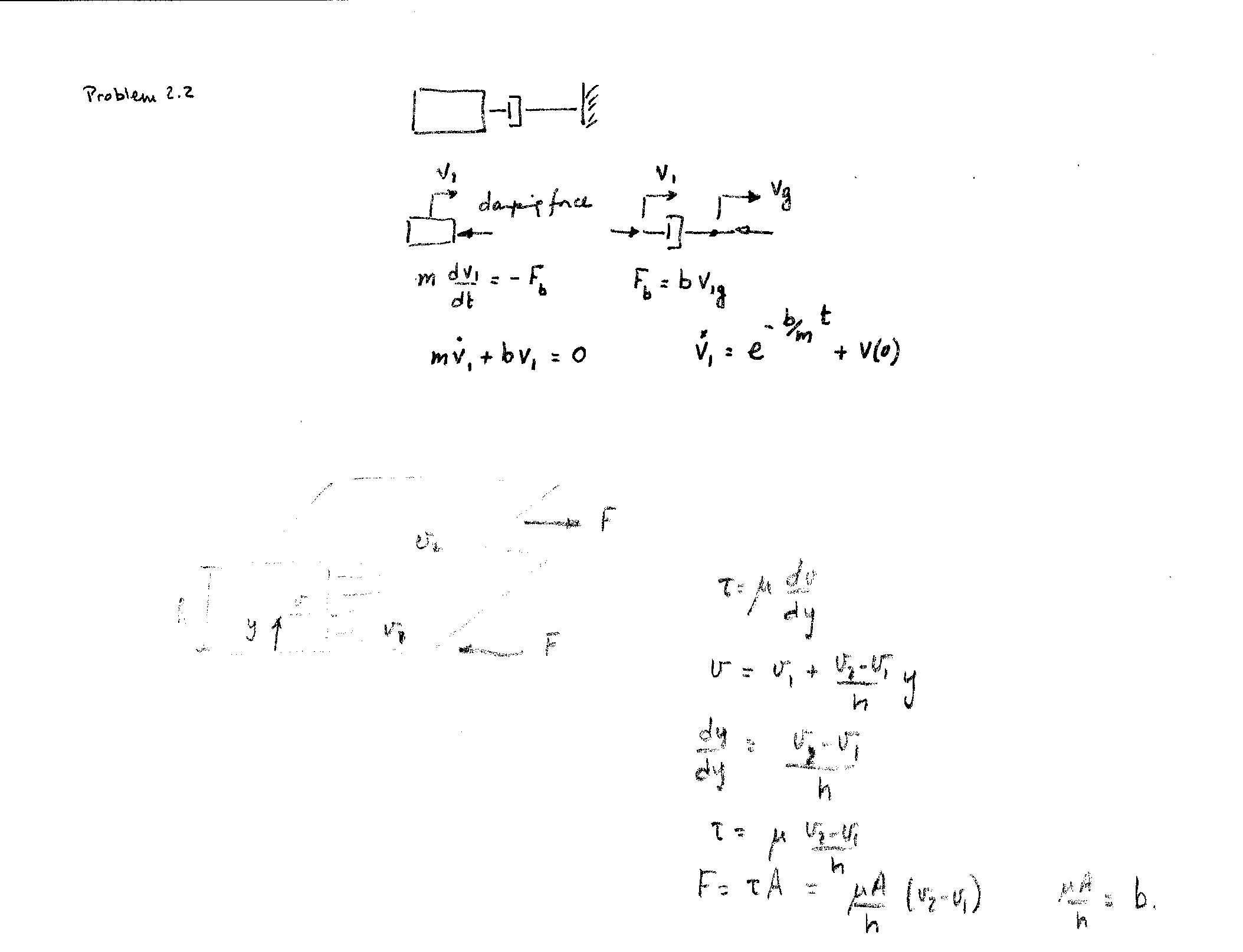
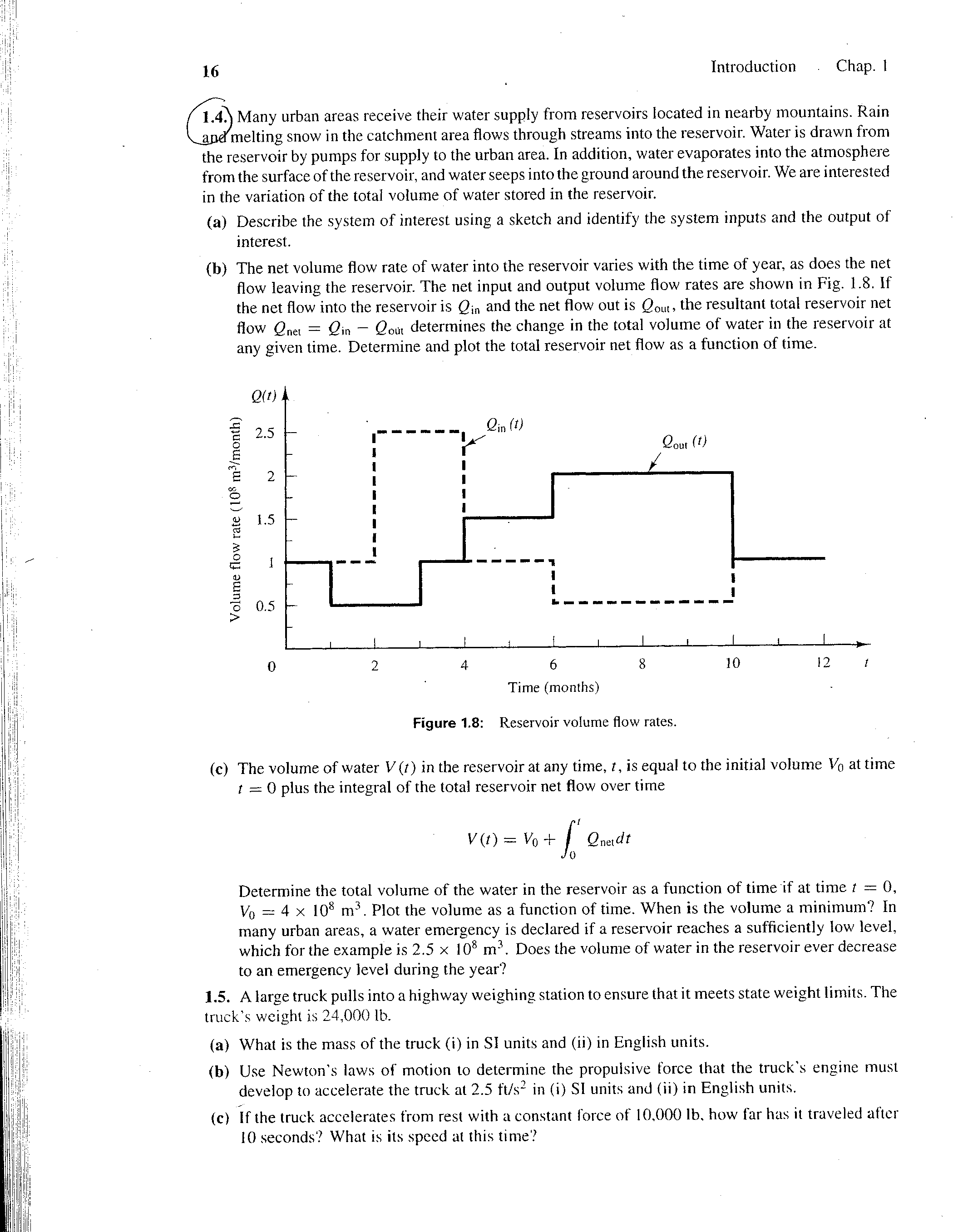
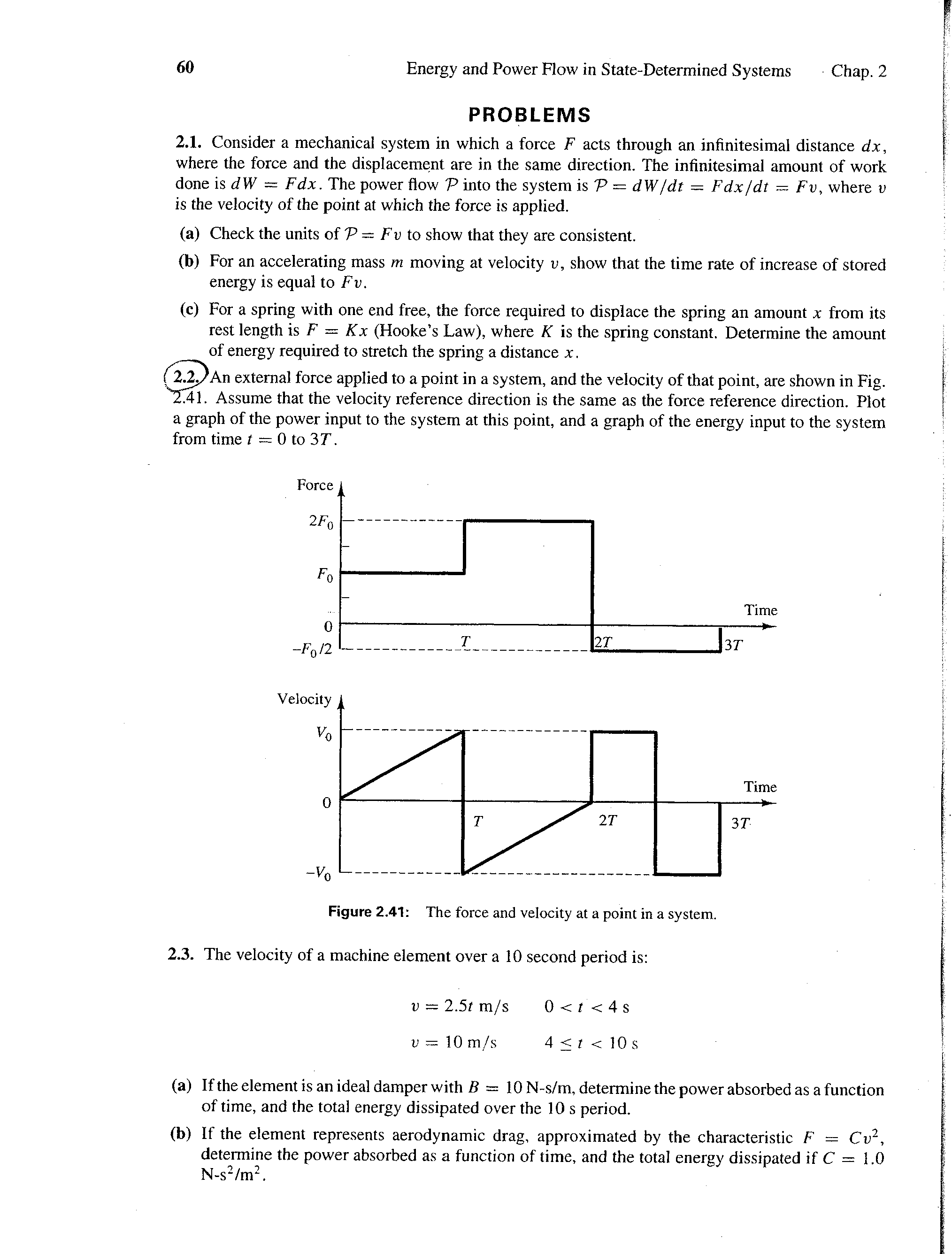
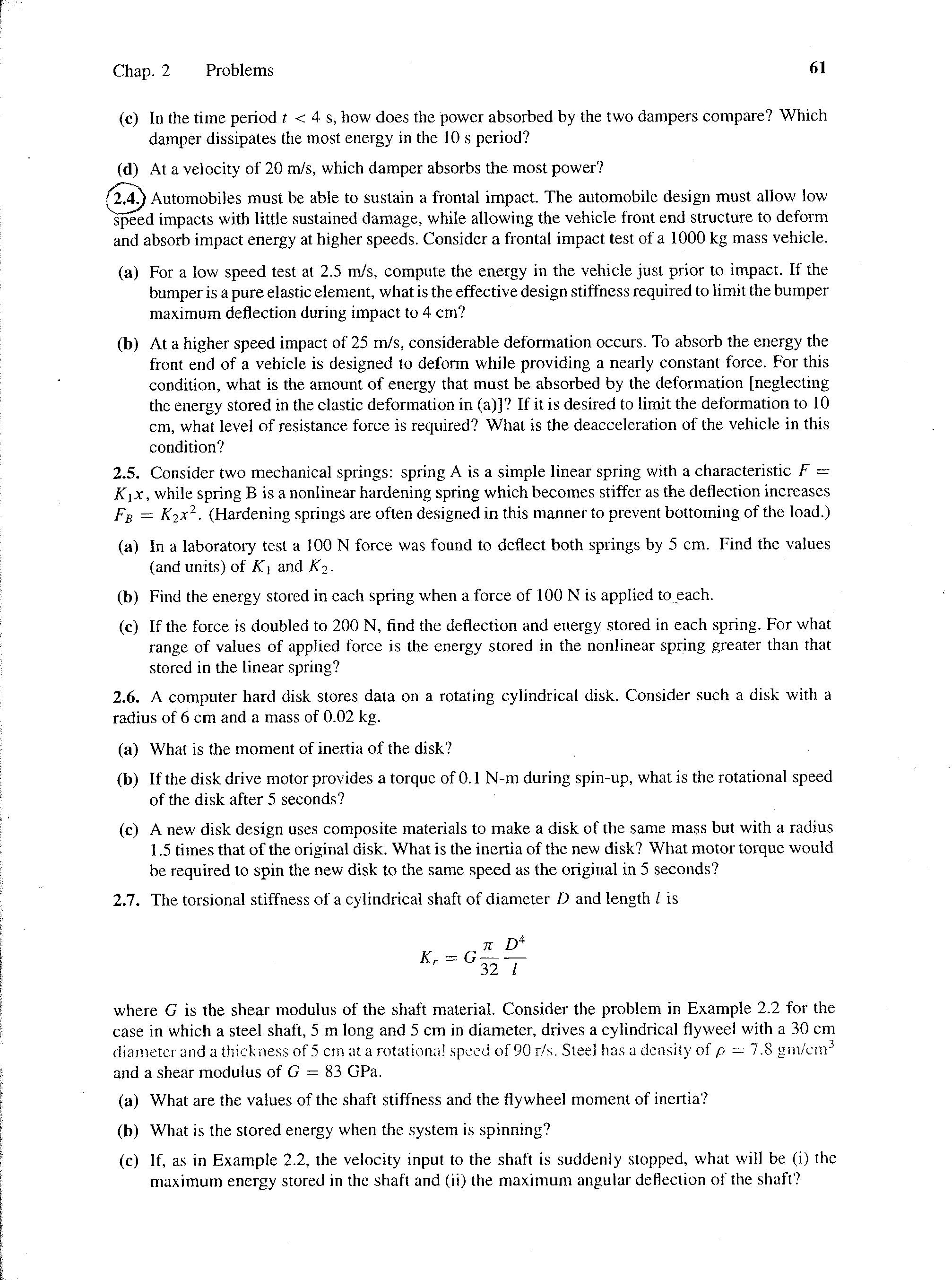
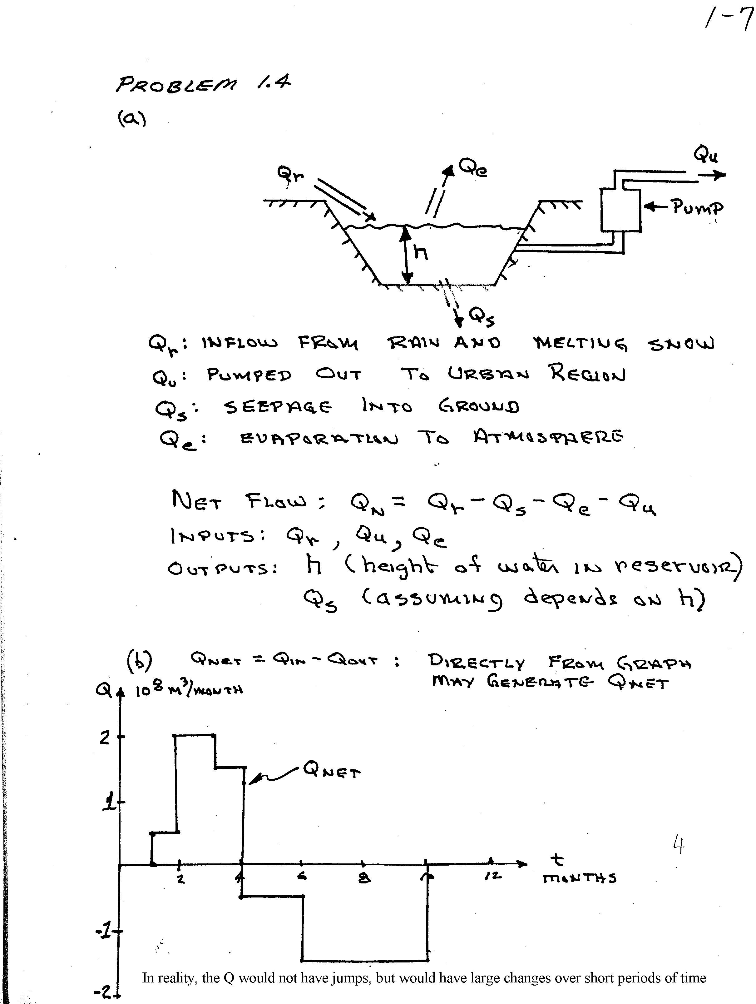
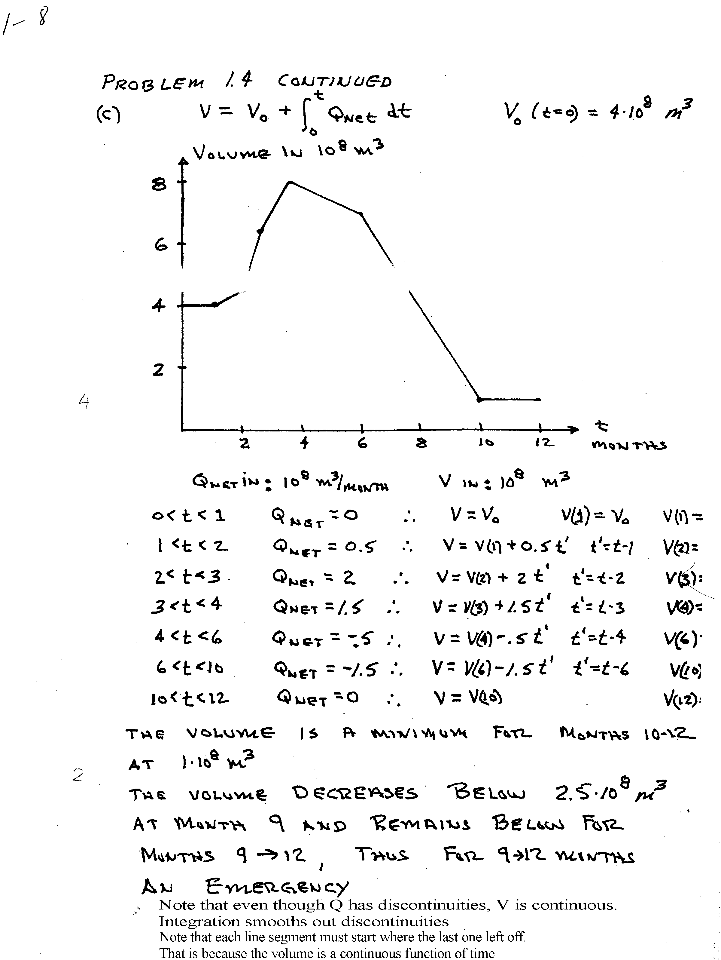
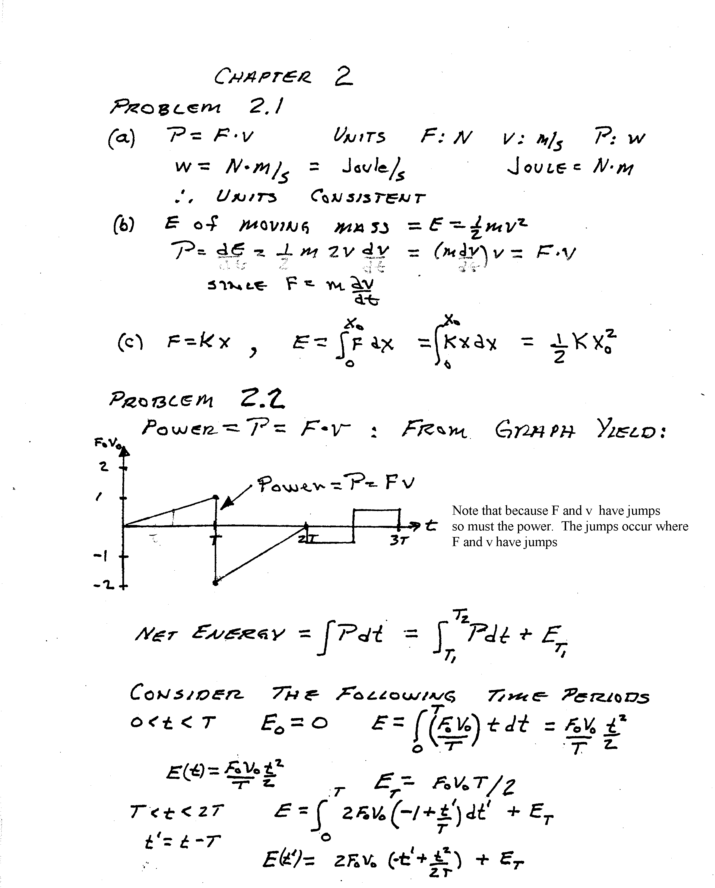
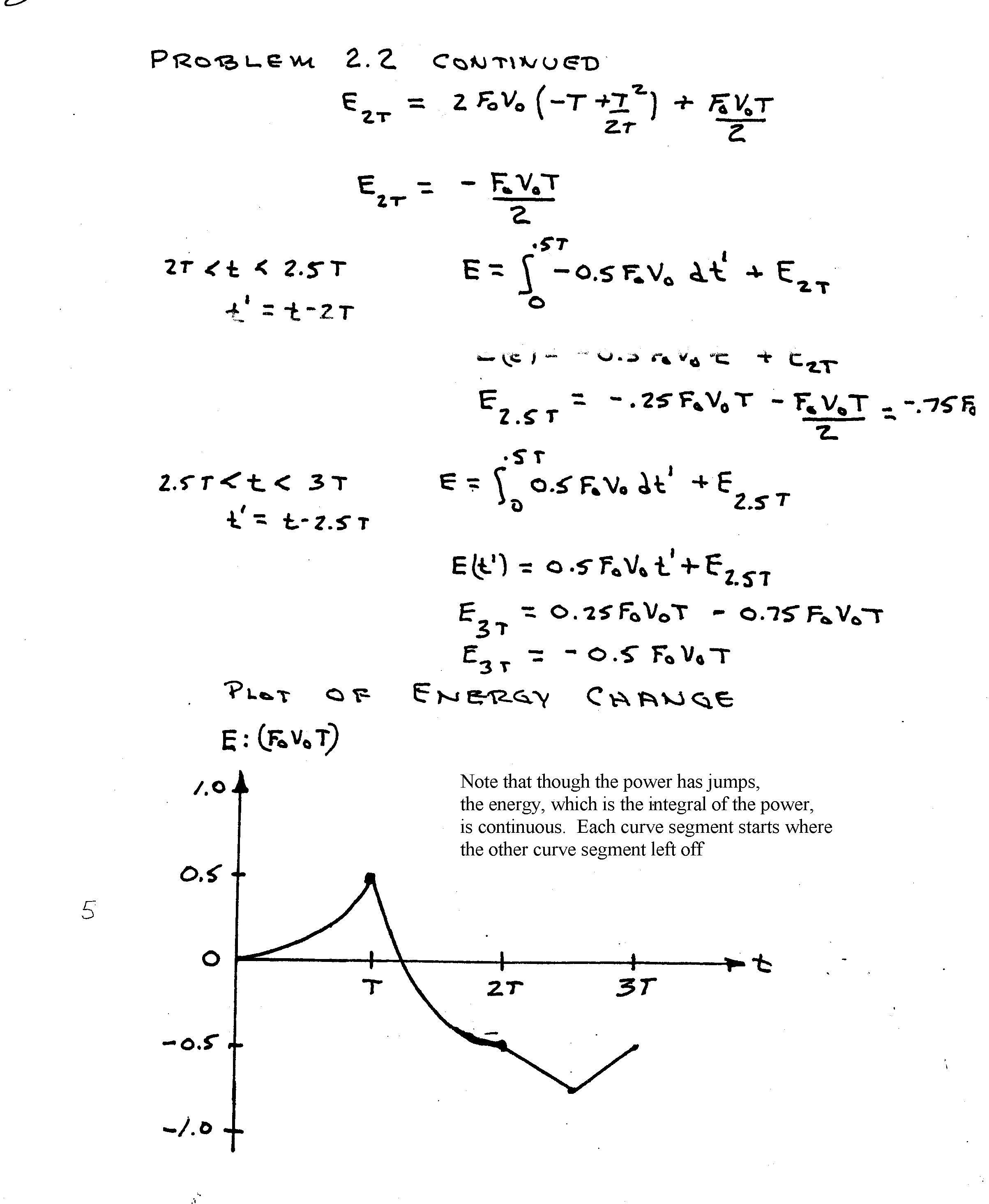
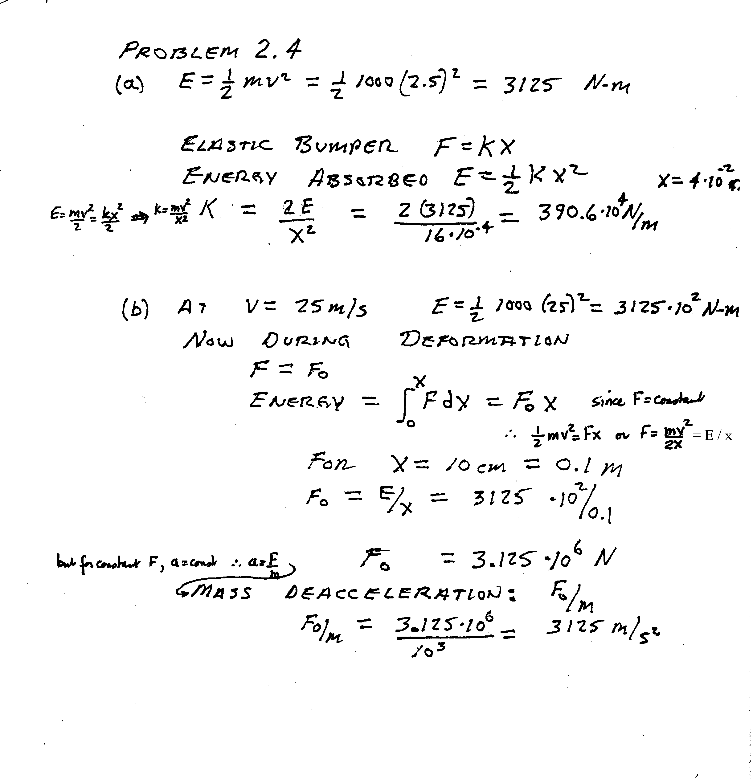
HW # 1 is: Problems 1.1, 1.4, 2.2, 2.4 from your Rowell and Wormley books. It will be due when announced in class.

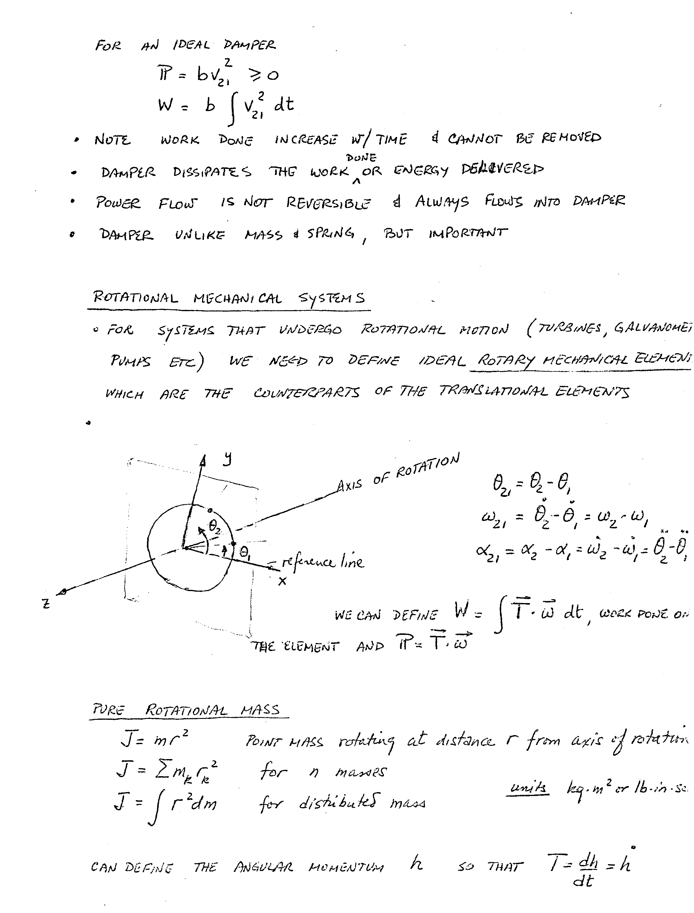
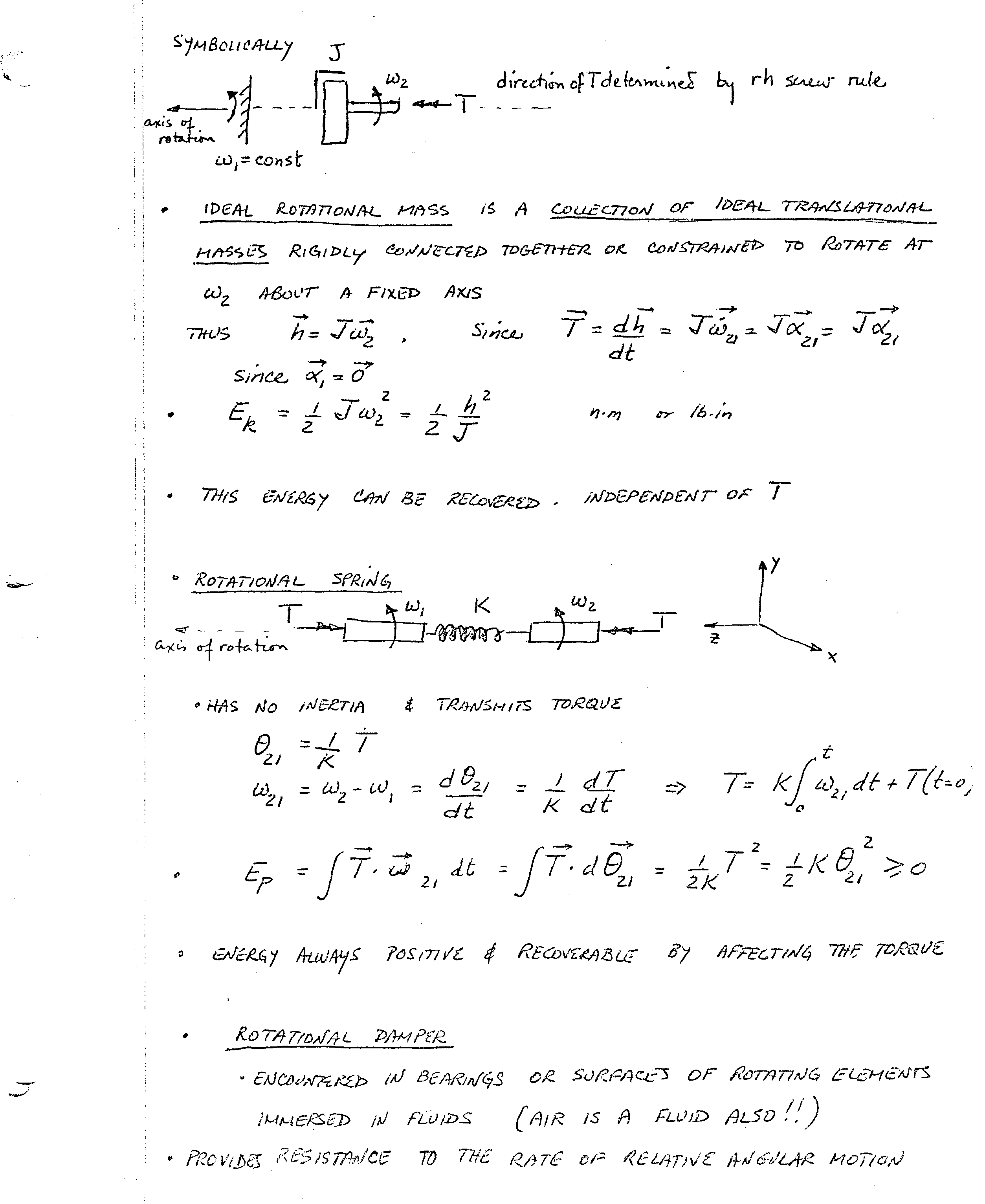
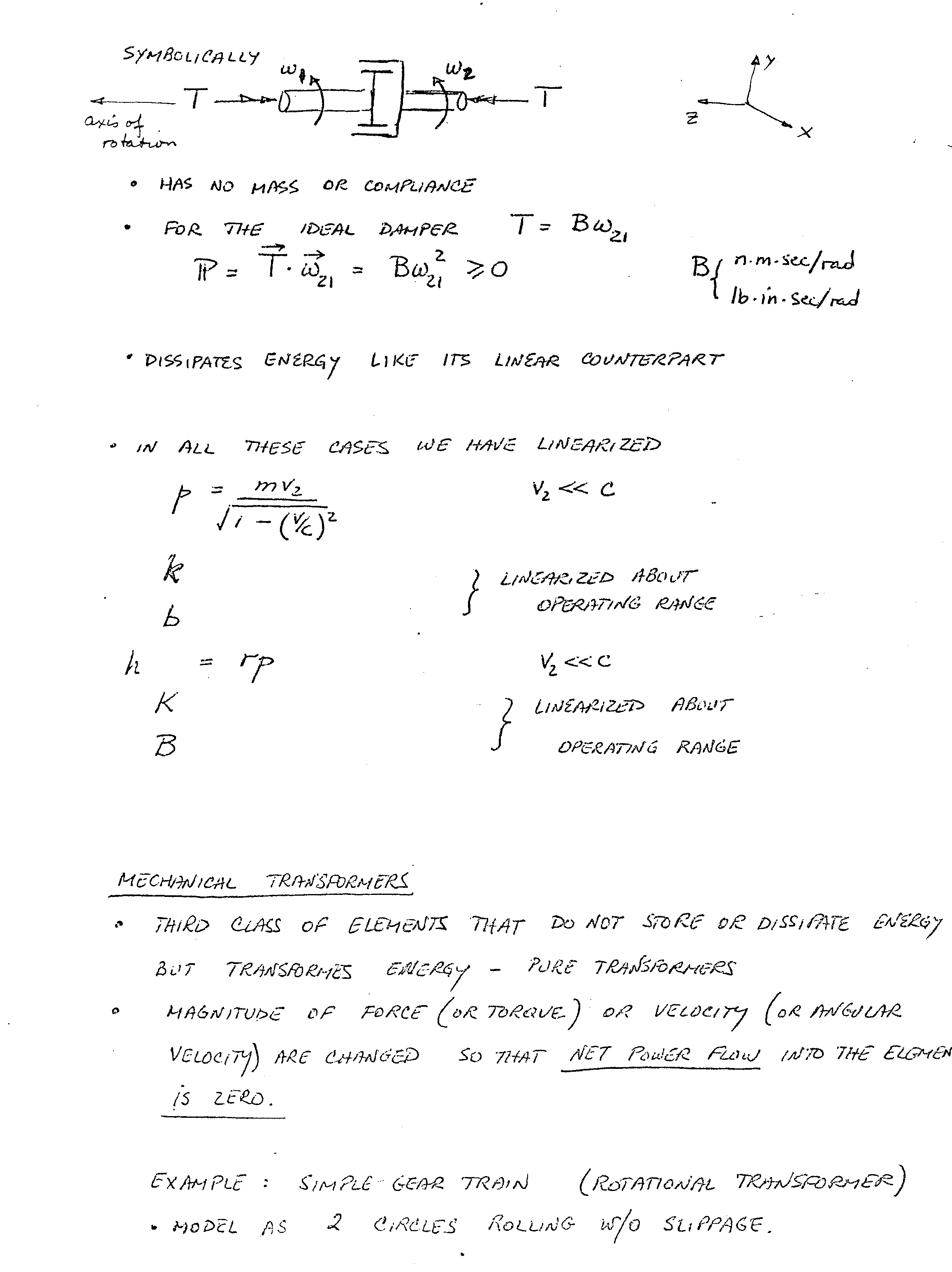
Here is the material that goes with Lecture 4 video: The video covers the rotational mechanical system elements page12, page 13, page 14, page 15, page 16, page 17,

Here is the material that will go with Lecture 5 video: The information on electrical elements begins at the end of page 17 and continues on page 18, page 19, page 20,

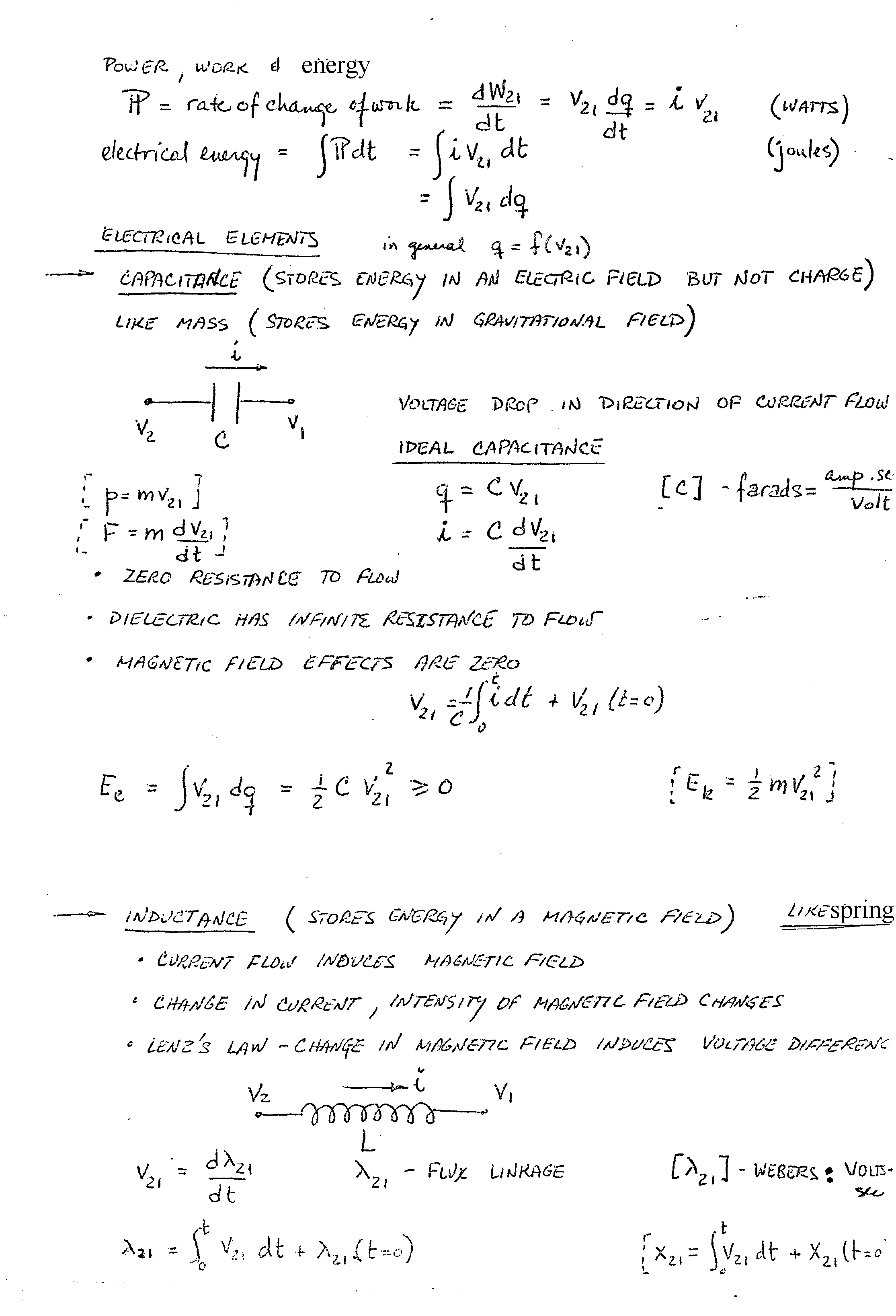
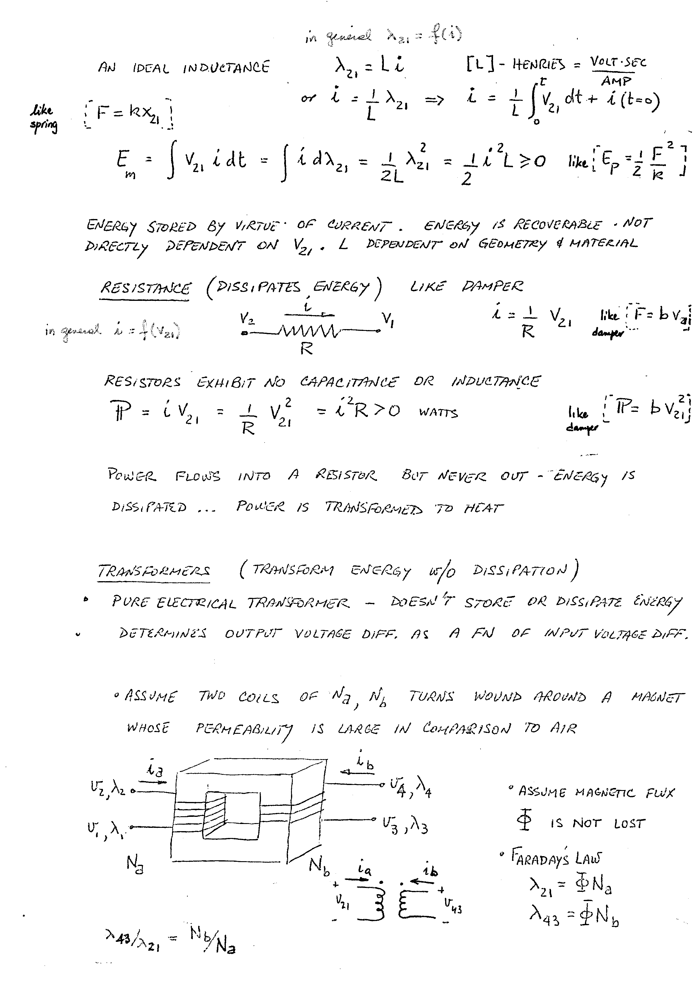
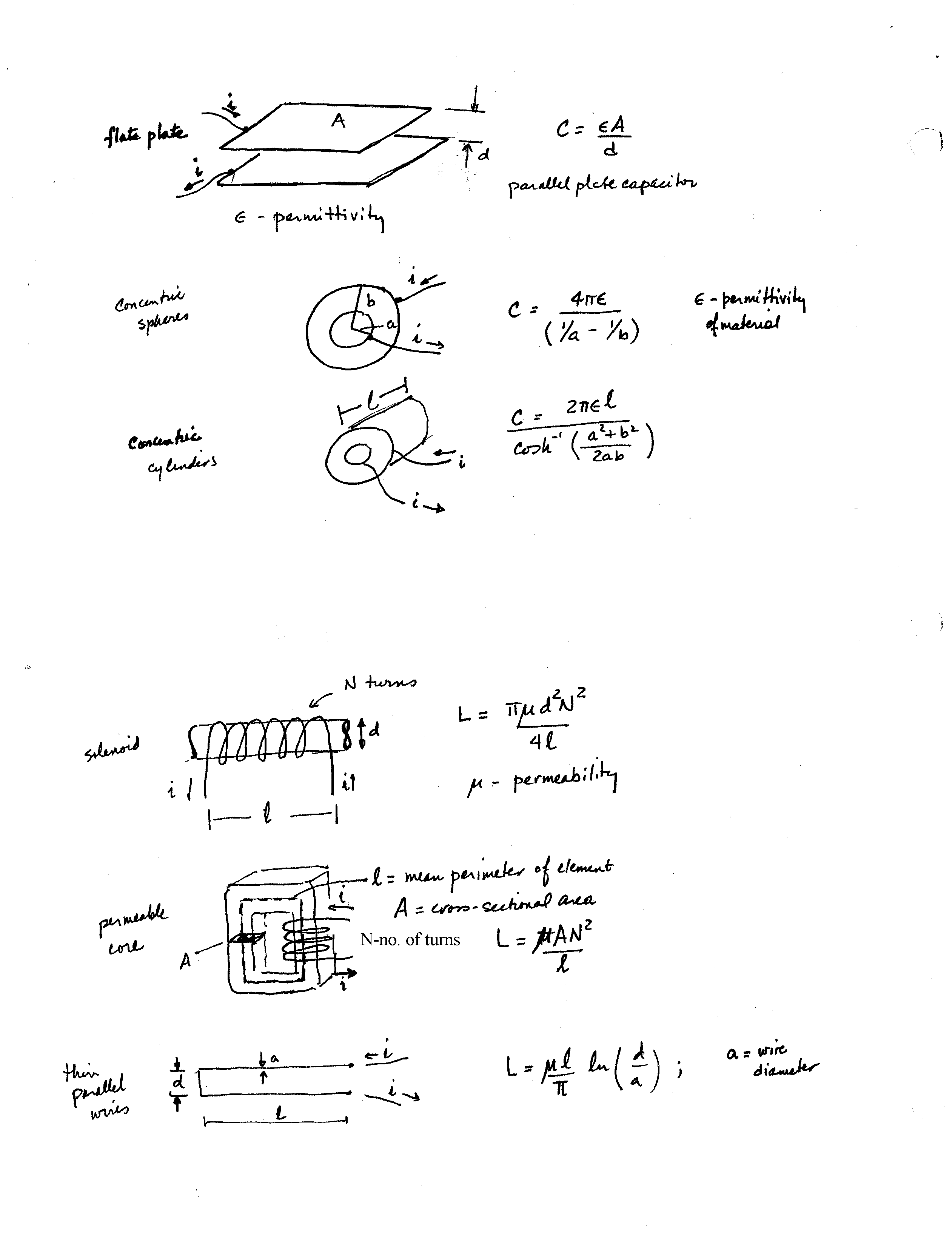
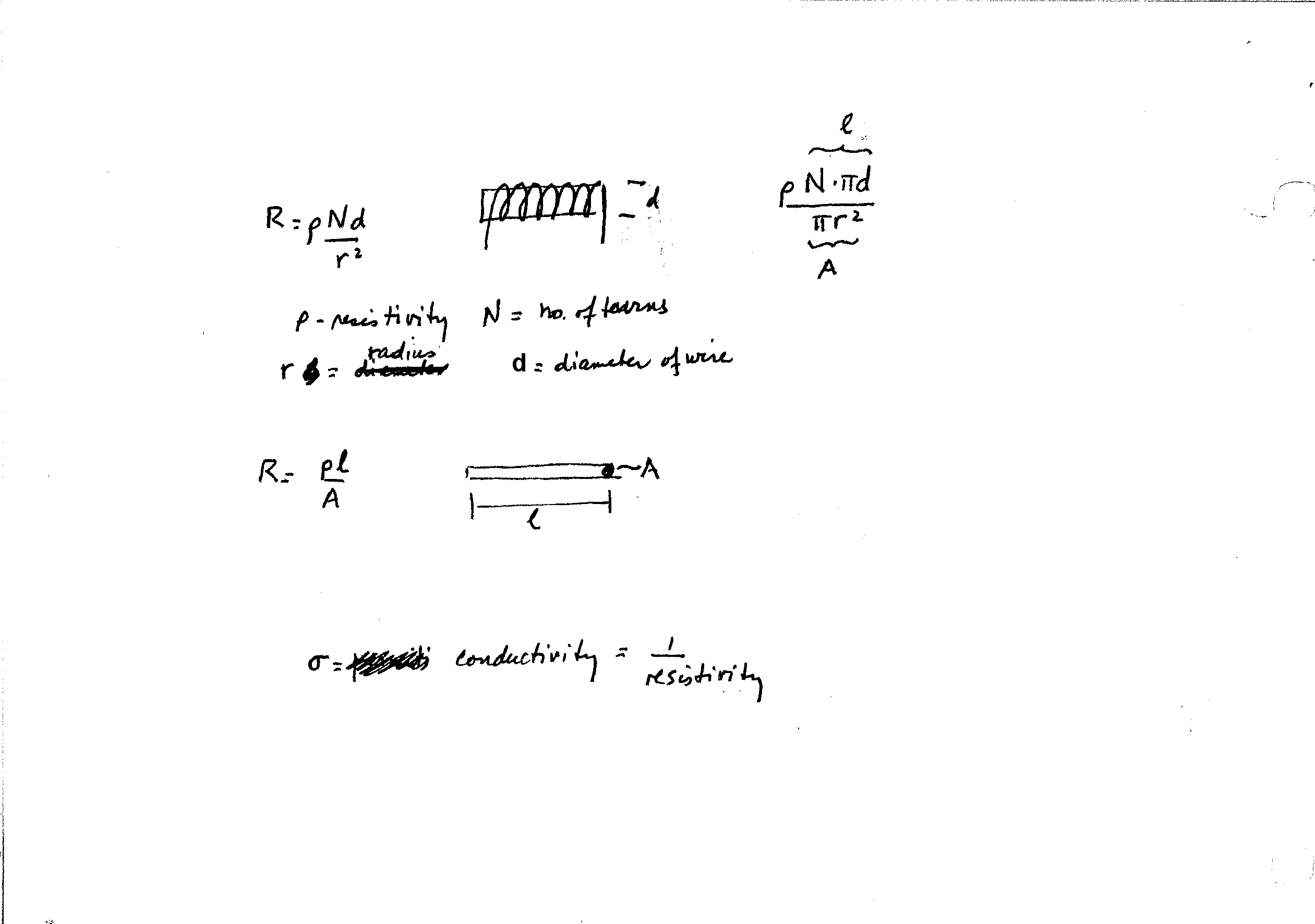
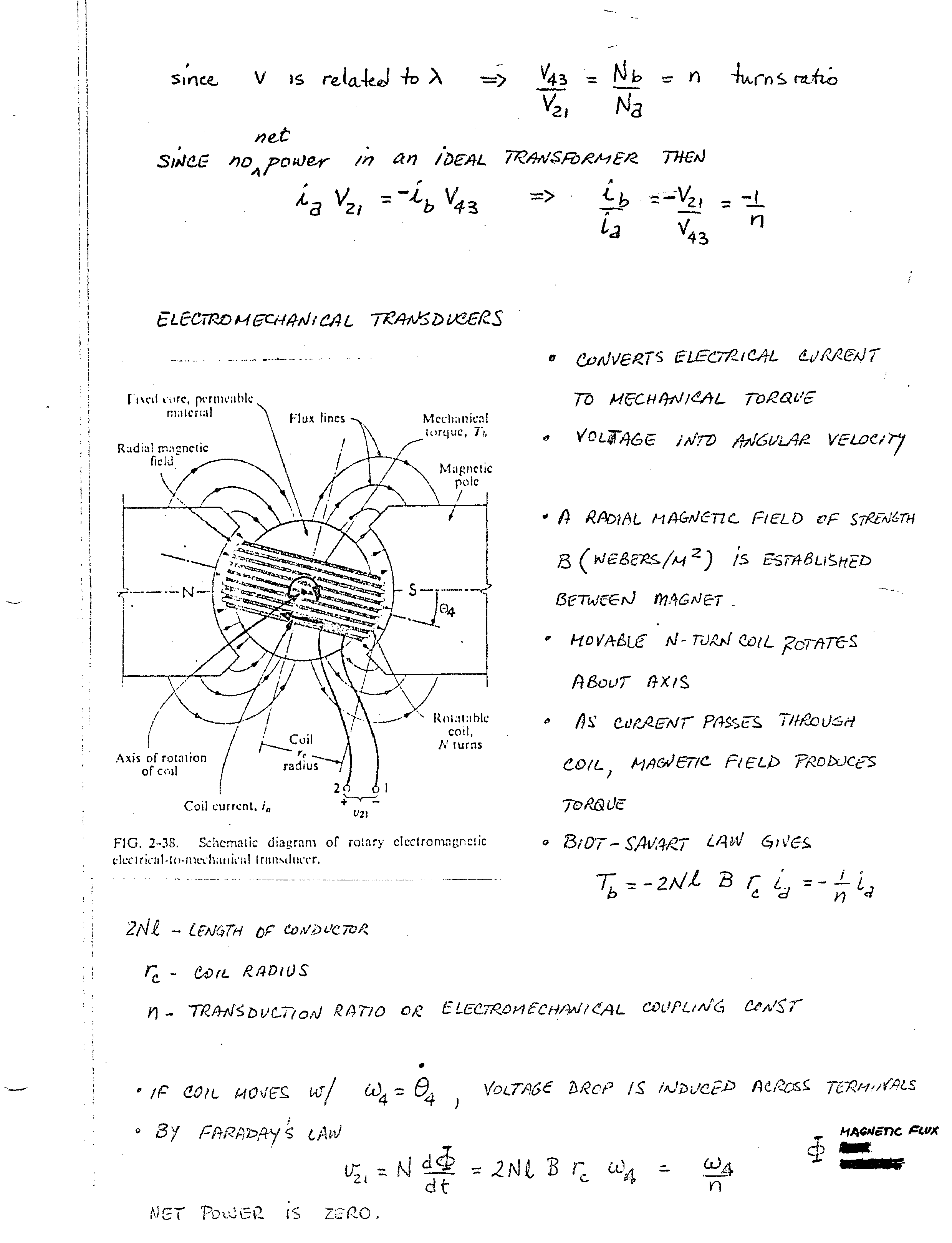
The information on electrical elements: capacitors, inductors and resistors are like electrical “masses”, “springs” and “dampers”. Please read and understand. The material will not be covered in depth in class but you will be responsible for it. I will skim over the material to cover the main elements, transformers and transducers. Just note the similar way we can describe electrical elements.

Continue reading chapter 6 on transducers in one energy domain (transformers) and transducers in multi energy domains (transducers)

Lesson 6 continues the materials discussed in Lecture 5: examples with electrical elements, examples with electrical elements 2, page 21,

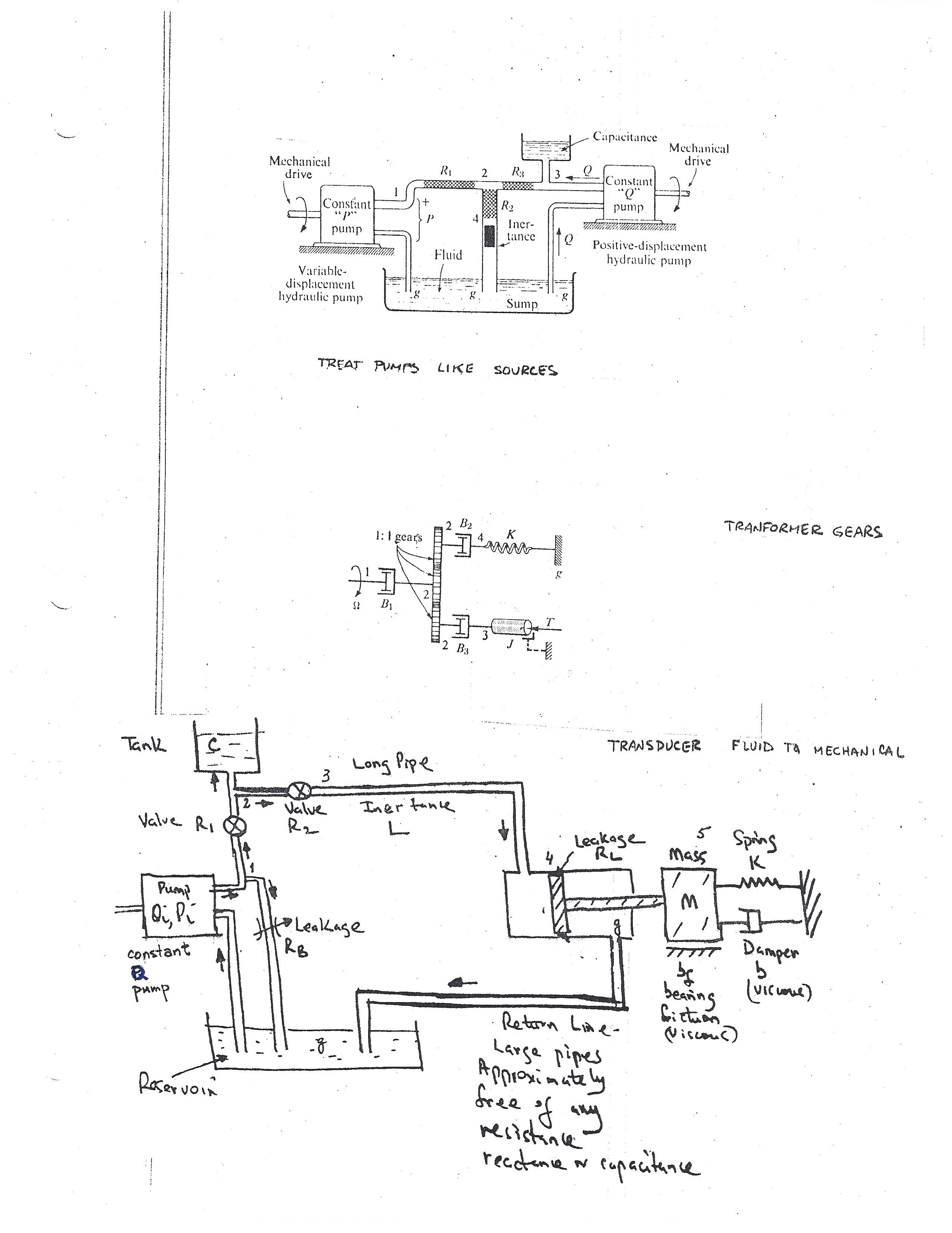
Here are the pages that go with Lecture 6 on Fluid systems: page 22, page 23, page 24, page 25, page 26, page 27,

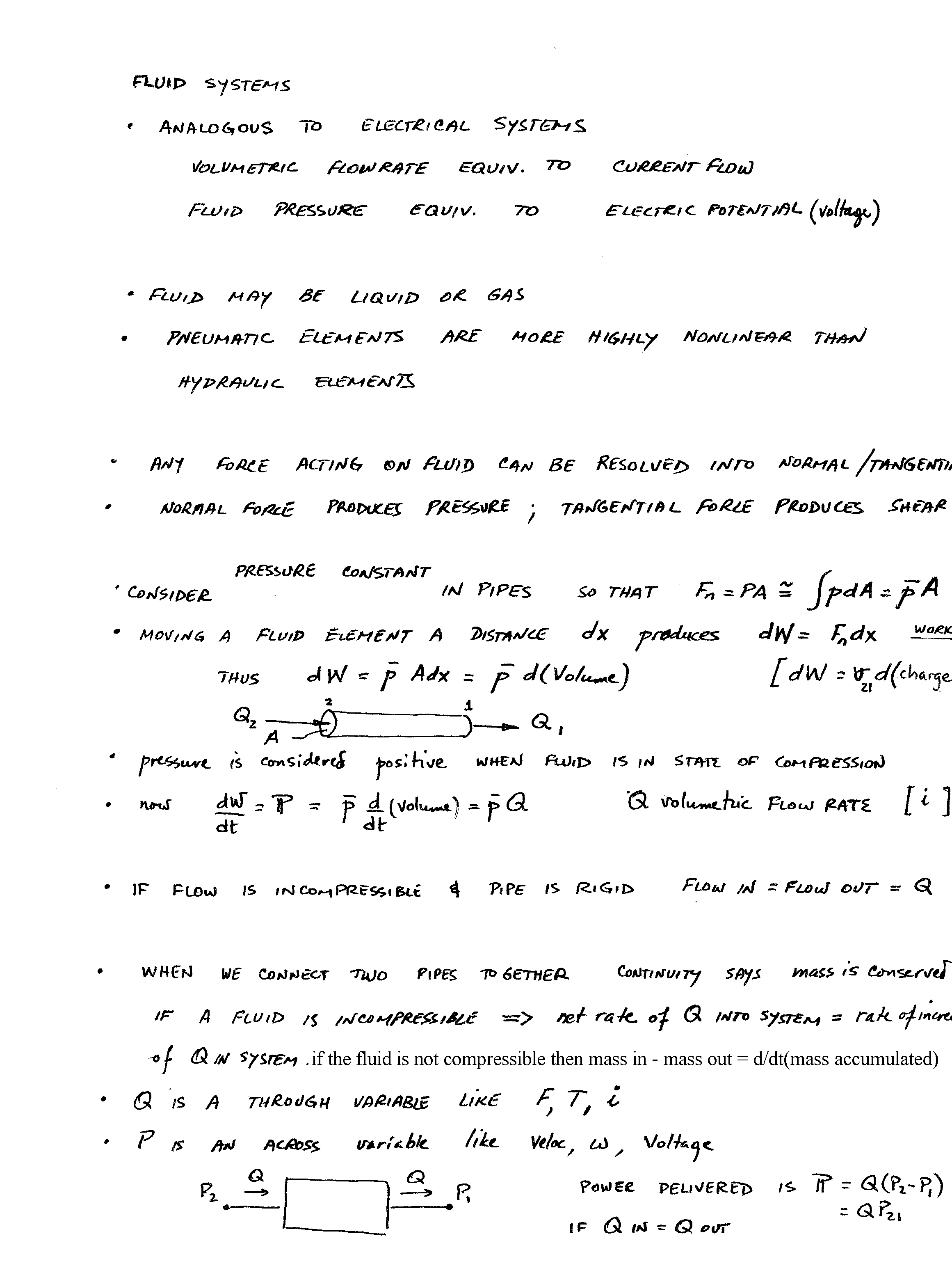
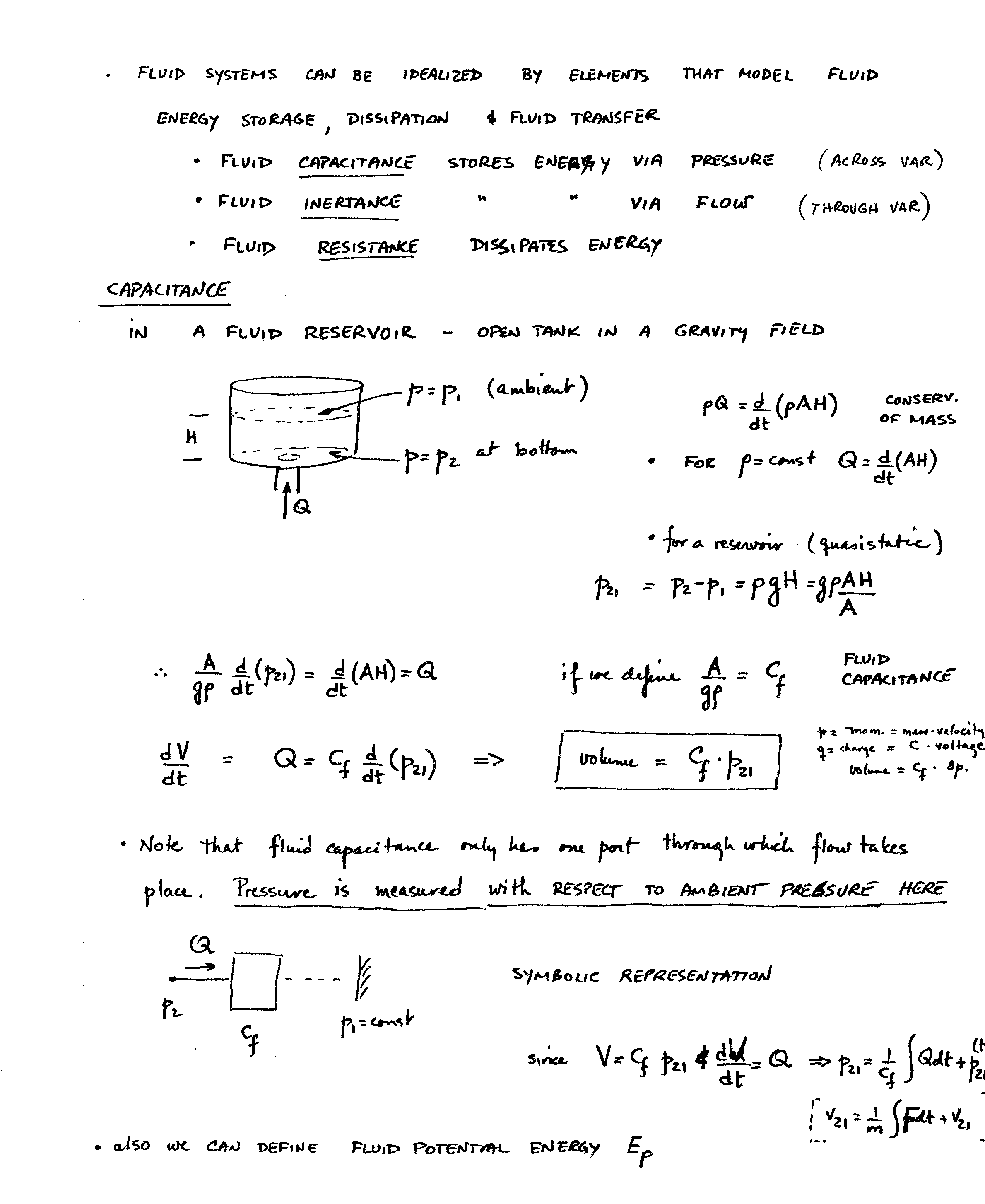
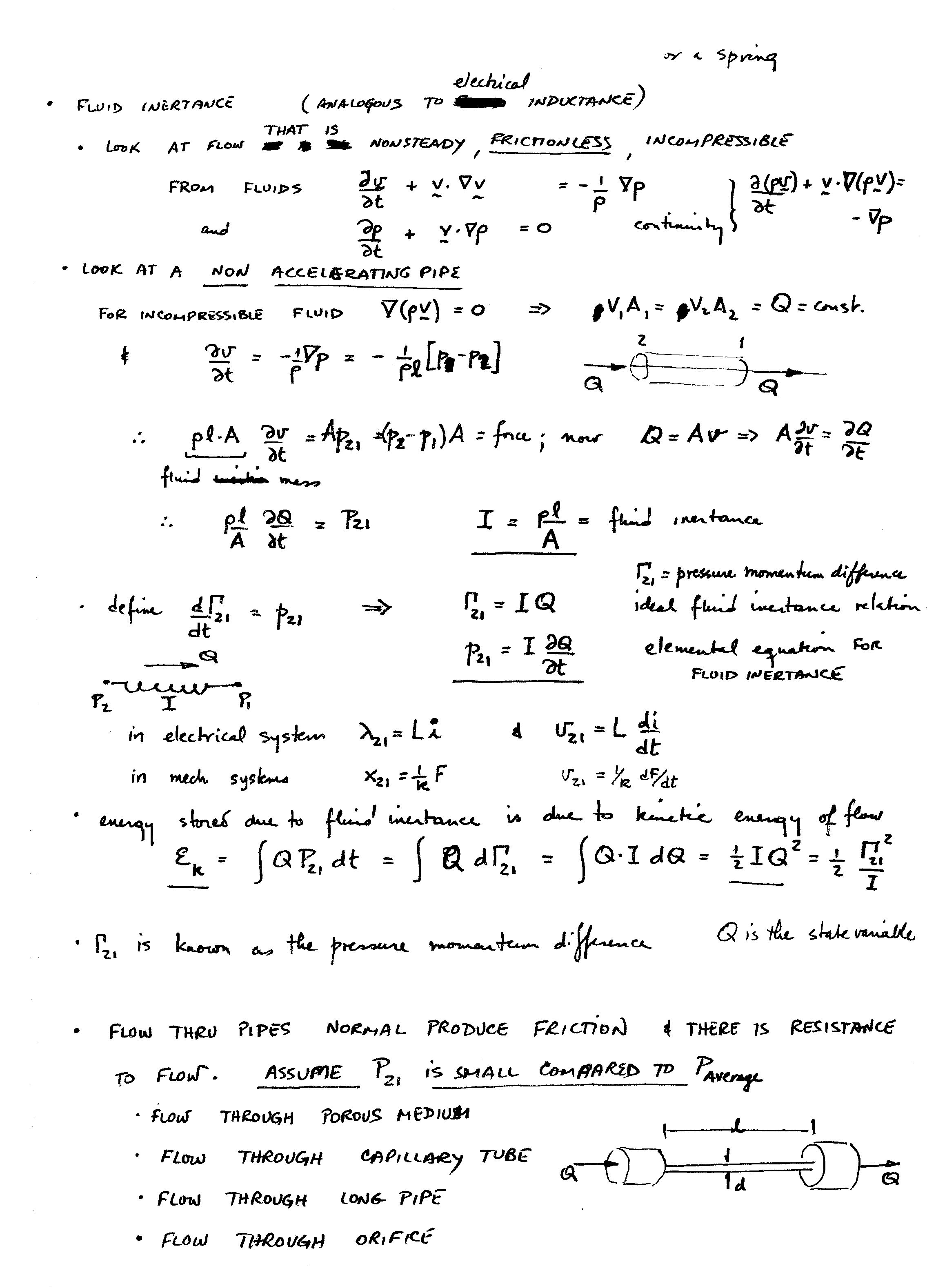
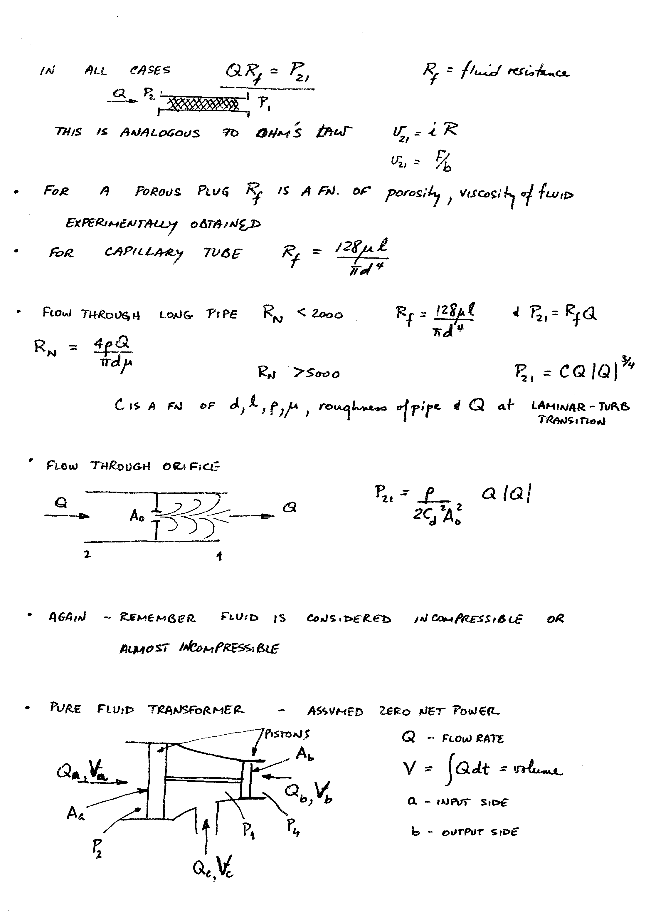
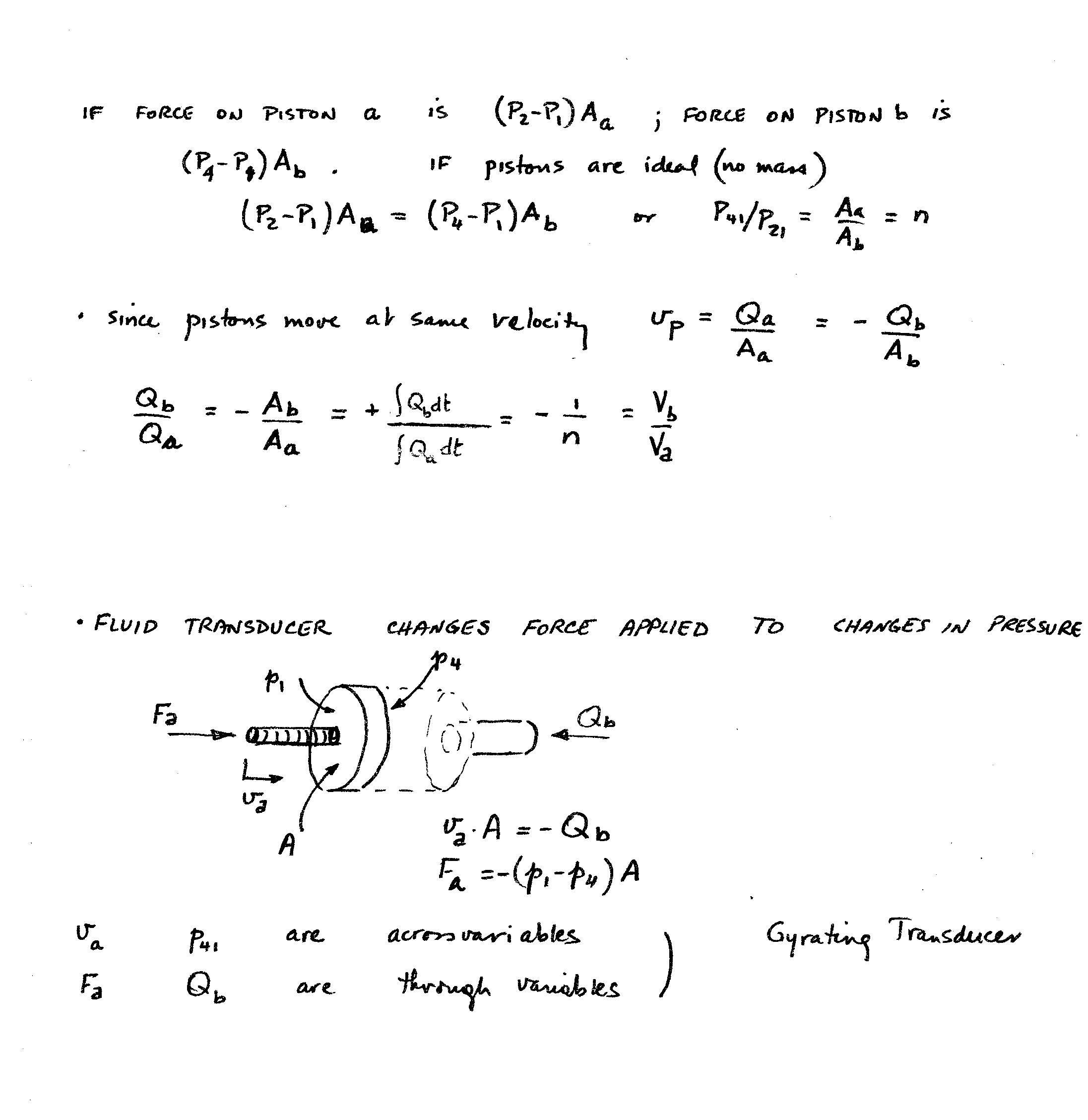
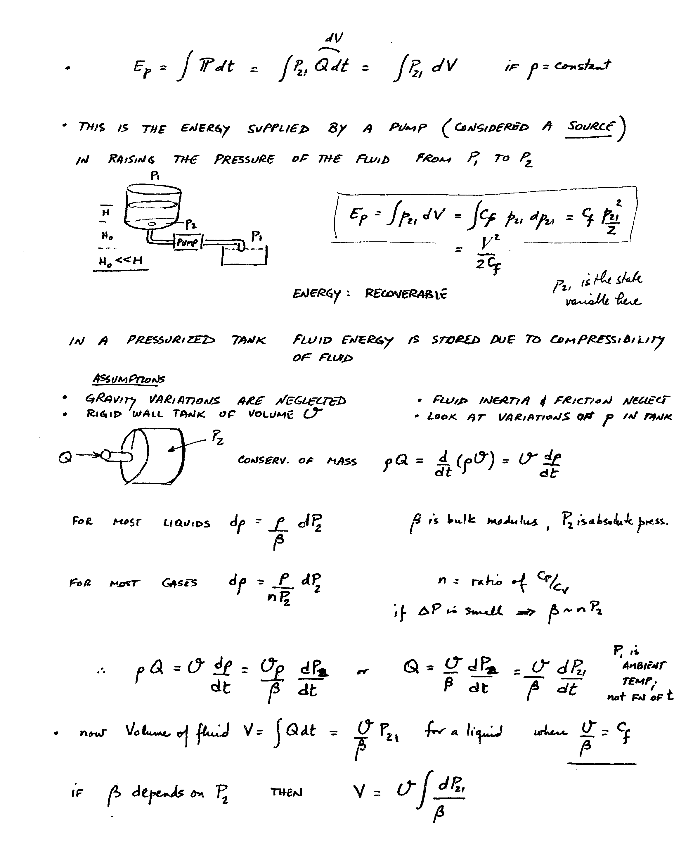
Here is the material that will go with Lecture 7 video that covers more on the fluid systems and also begins thermal systems as well: page 26, page 27, page 28, page 29, page 30,

Here is the material that will go with Lecture 8 video: page 30, page 31, page 32, page 33, page 34, example solution

Please read chapters 3 and 4 of Rowell and Wormley book on system graphs. We will start talking about those during the next lecture.

Here are the Problems 1.1, 1.4, 2.2, 2.4 and the solutions: problem 1, problem 2a 2b, problem 3a 3b, problem 4

Having completed the understanding of the basic ideal elements in each type of system and their similarities, we now begin by showing you how to take physical systems, simple ones first-then more complicated ones, and construct a system graph made up of the elements we just discussed. The videos and pages from this point forward deal with this new topic.

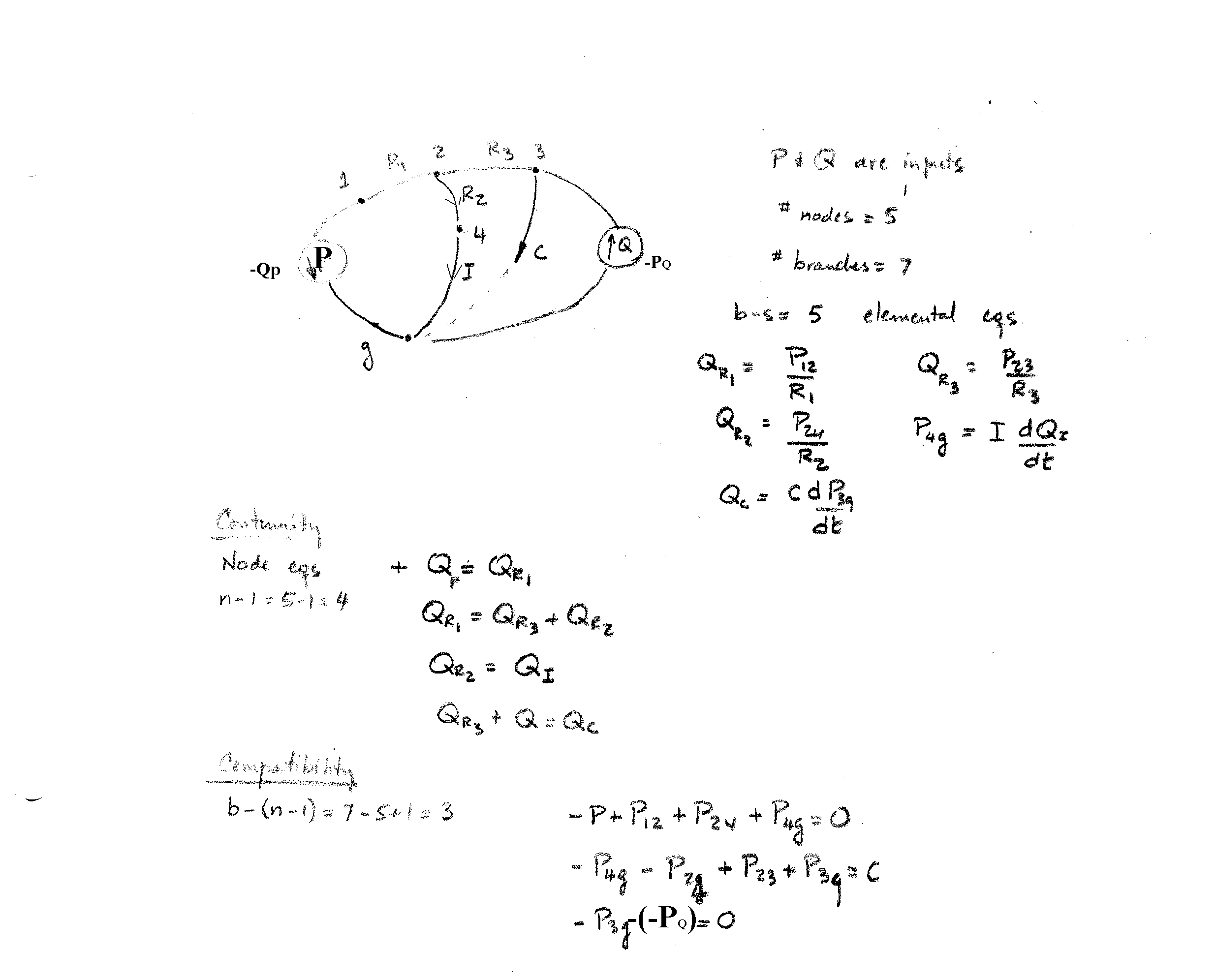
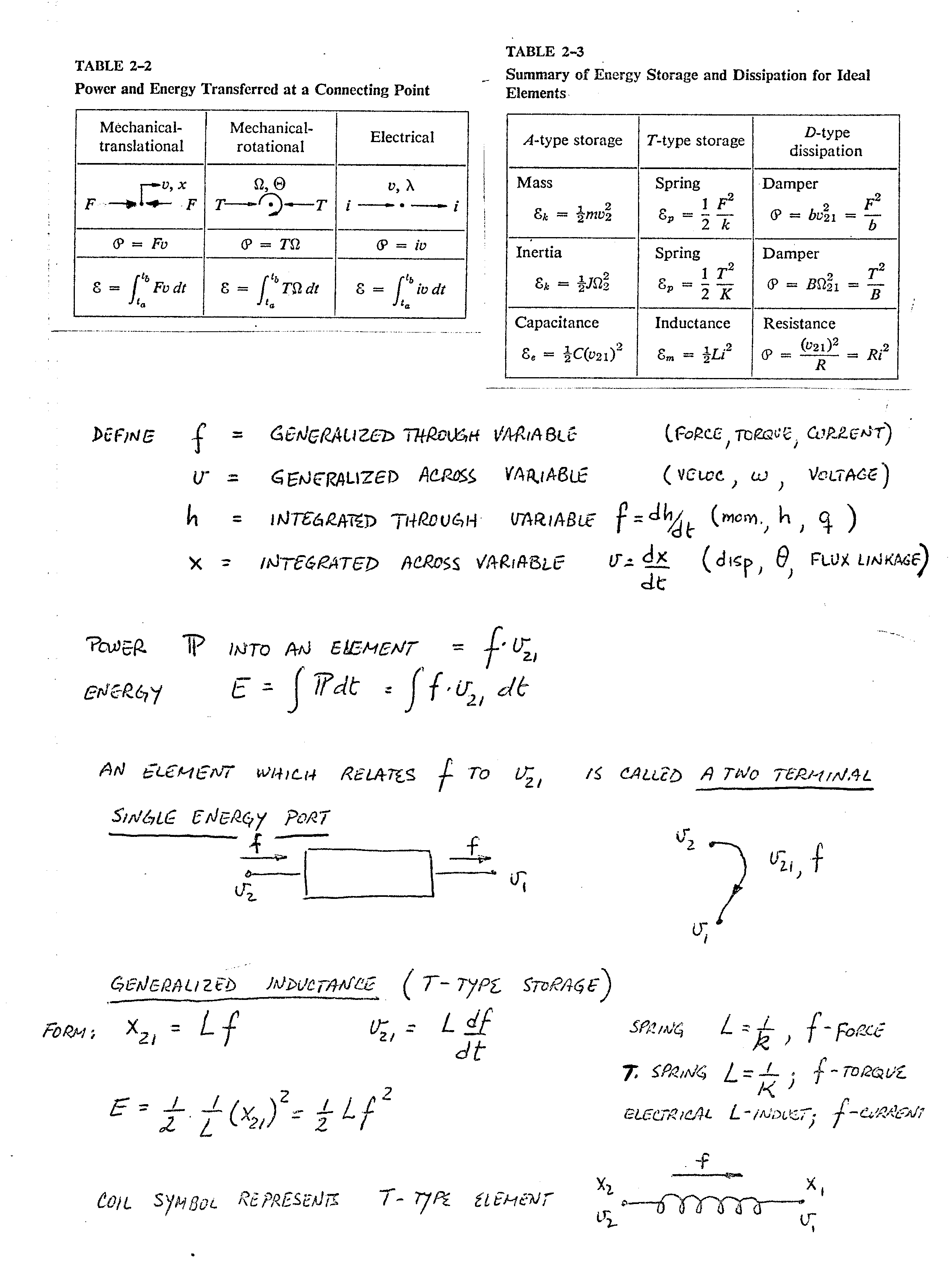
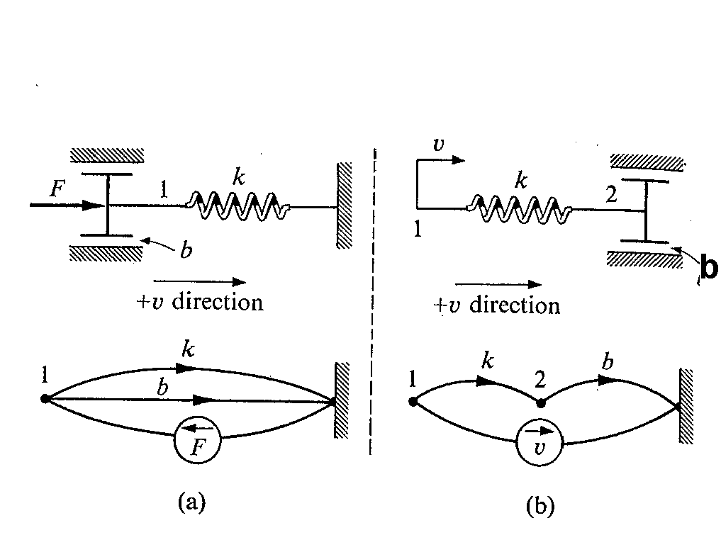
Here is the material that goes with Lecture 9 video: page 36, page 37, page 38, page 39, page 40, page 41, page 42. This material deals with system graphs and the governing equations for through variables and across variables.

Here is the material that goes with Lecture 10 video: page 42, page 43, page 44, page 44solution, page 45-46 examples, page 45-46solns. Here is the material that goes with Lecture 10partb video: page 47, page 48, page 49,

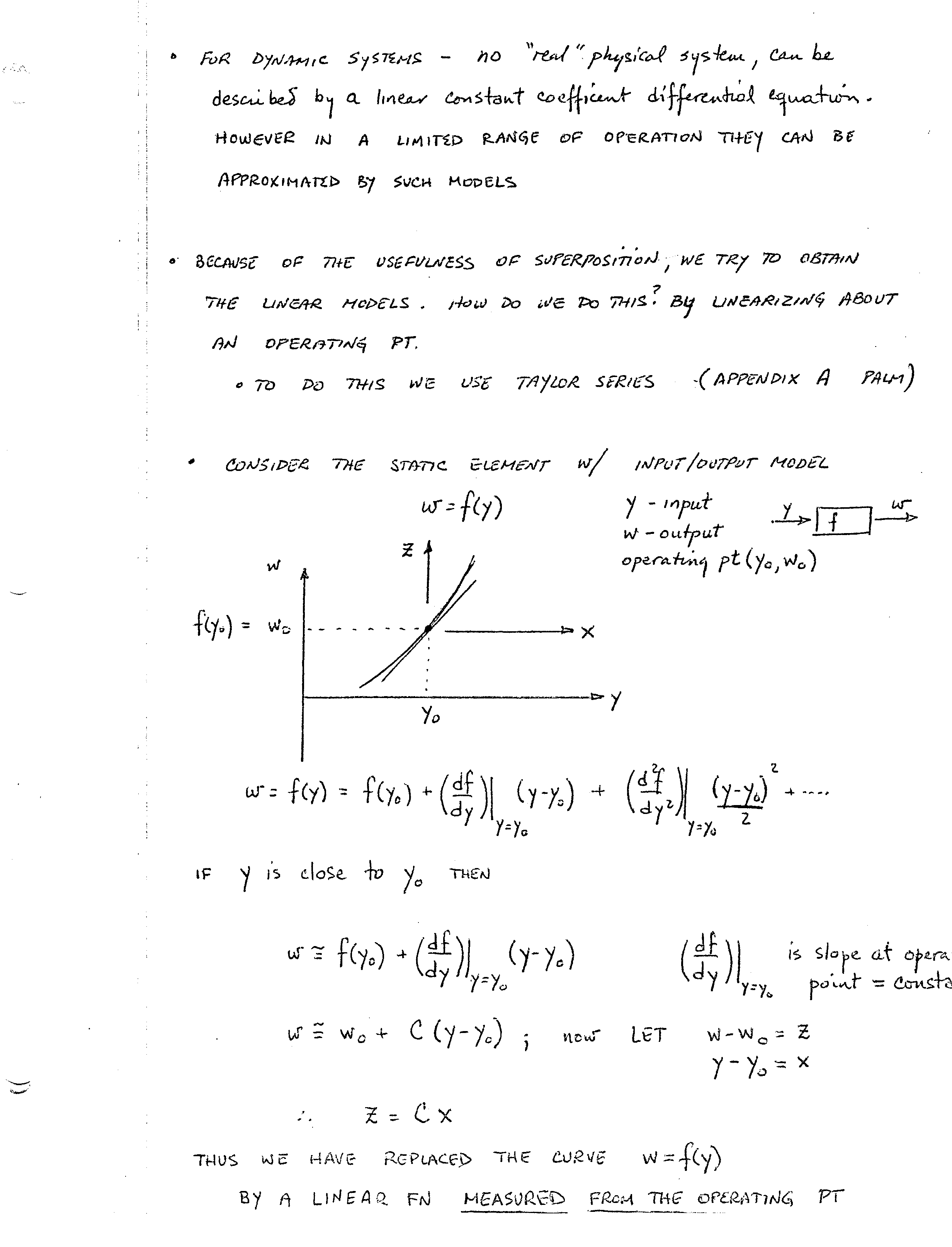
First Exam is announced for the 9th of October. It will cover definitions given in the first handout, your knowledge of the equations for the different systems’ ideal elements, similarities and differences with thermal systems and also know how to work out linearization problems.

Here is the material that goes with Lecture 11 video: page 49, page 50, and page 51. Here is the material that goes with Lecture 11 part b video: page 52, page 53, and page 54. The last portion deals with an example that involves a transformer and how to represent it in a system graph.

Here are your choices for project (the ones with strikethrough are already taken):

~~Foot Driven Potter’s wheel~~

~~Normal two wheel Bicycle operation~~

~~Simplified Operation of a grandfather’s clock~~

~~car braking system (from foot brake to wheel) as mentioned in class~~

electric shaver

~~Foot driven paddle wheel boat~~

~~animal powered grinding mill (used in 3^rd world countries to grind wheat)~~

~~water powered grinding mill (as found in the northeast in the late 1700’s-early 1900’s)~~

~~Windmill operation/Wind turbine operation~~

~~windshield wiper operation~~ (check patent to understand how it works)

~~manual garage door system where human pulls on a chain to lift the door to the garage~~

~~car steering system (steering wheel to tire wheels) --torque you apply to steering wheel is input~~

~~manually operated dumbwaiter systems~~

spinning wheel used to spin sheep’s wool into thin thread or yarn

~~fishing pole reel mechanism~~

~~hand mixer~~

ANY OTHER ACCEPTABLE PROJECT I APPROVE

Please note that choice of projects are first come first served basis.

Project Information:

You will be expected to work as a part of a team of 4. We have 55 students in the class-therefore there should be 14 projects (14x4). PLEASE SEND ME THE NAMES OF THE 4 STUDENTS and YOUR TOP 3 PROJECTS IN CASE YOU ARE CLOSED OUT OF THE ONE YOU WANT

You will be expected to produce and turn in a project report by Nov. 29 in a form similar to your lab reports. The report will include:

· An introduction detailing what you are planning to model, who your team members are and what they have contributed to the project;

· Modeling section in which you give the system you are investigating and the modeling of your system, and the assumptions you are making. You will show the elemental equations, nodal equations, path (loop) equations, the state variables, sources, and the state variable equations and the matrix form of those equations. You will be expected to explain the expressions for the constants you use in your elemental equations—this should come from the simplifying assumptions you make.

· A results section in which you detail the numerical equations you will be using to solve the problem, the parameters you will be using in your equations and where those parameters have been obtained, the graphs of the state variables as a function of time, the outputs you want to find as a function of time;

· and finally a Discussion of your results. Also discuss the step-size you use and its effect on the accuracy of the results

· What have you learned from the project and what would you suggest for future work to understand the results more fully.

You will need to vary at least 3 parameters to see the effect of parameter variation on your solutions. Your discussion section should be in depth—how each parameter change affects the overall results. All graphs should be properly labeled (units, what are the parameters tested).

Additional to the parameter variations above, you will be expected to vary the source variables.

In all your projects you probably have one source (maybe more). Please take one of the sources in the form A + B sin(omega*t) where A is the amplitude of the source strength and B is the variation in the source strength and omega is the frequency of the variation. Please vary at least two of these variables; for instance you can take B as being 0.1 A, 0.3 A; or omega as being some value between 0.5 pi to 2 pi.

PROJECTS ARE DUE TO MY OFFICE (EC3442) BY Nov. 29 by 3pm. YOU MUST GIVE ME THE PROJECTS, NOT SLIDE THEM UNDER MY DOOR. ITEMS SLID UNDER MY DOOR WILL NOT BE EVALUATED AND THE TEAM THAT DOES WILL GET A ZERO; SO PLEASE FOLLOW INSTRUCTIONS.

Please note that our first quiz will be on Wednesday, October 9 and will cover the similarities and differences between systems we have discussed. The first quiz will test you: regarding thru, across variables, integrated thru and integrated across variables, energy expressions for the different types of systems we have discussed (linear mechanical, rotational mechanical, electrical, fluid and thermal), definitions from first handout.

You will not be allowed any aids. The quiz will require you to remember things like definitions of transformers and transducers and the difference between a regular transducer and a gyrating transducer, major differences between thermal systems and the other systems.

Please note that the first major exam will be on October 24. In the exam you will be given a system and you will be asked to obtain the system graph and to derive the elemental equations (including transformer/transducer equations if any), the node equations (continuity), the path equations (loop, compatibility), and also some if not all the state equations (which will be covered shortly after system graphs are completed). Formula sheets will be allowed and will be discussed as we get closer to the exam date.

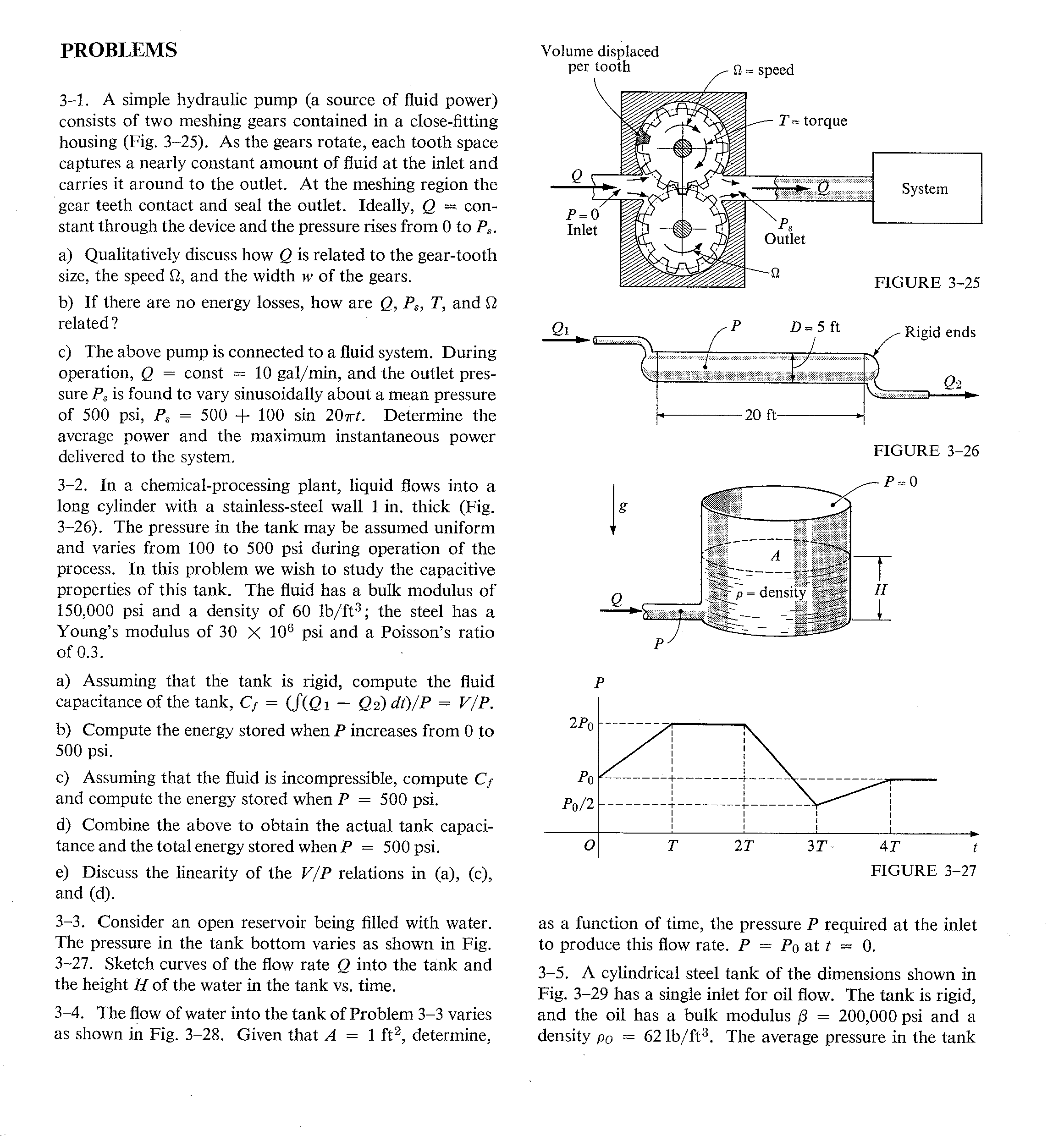
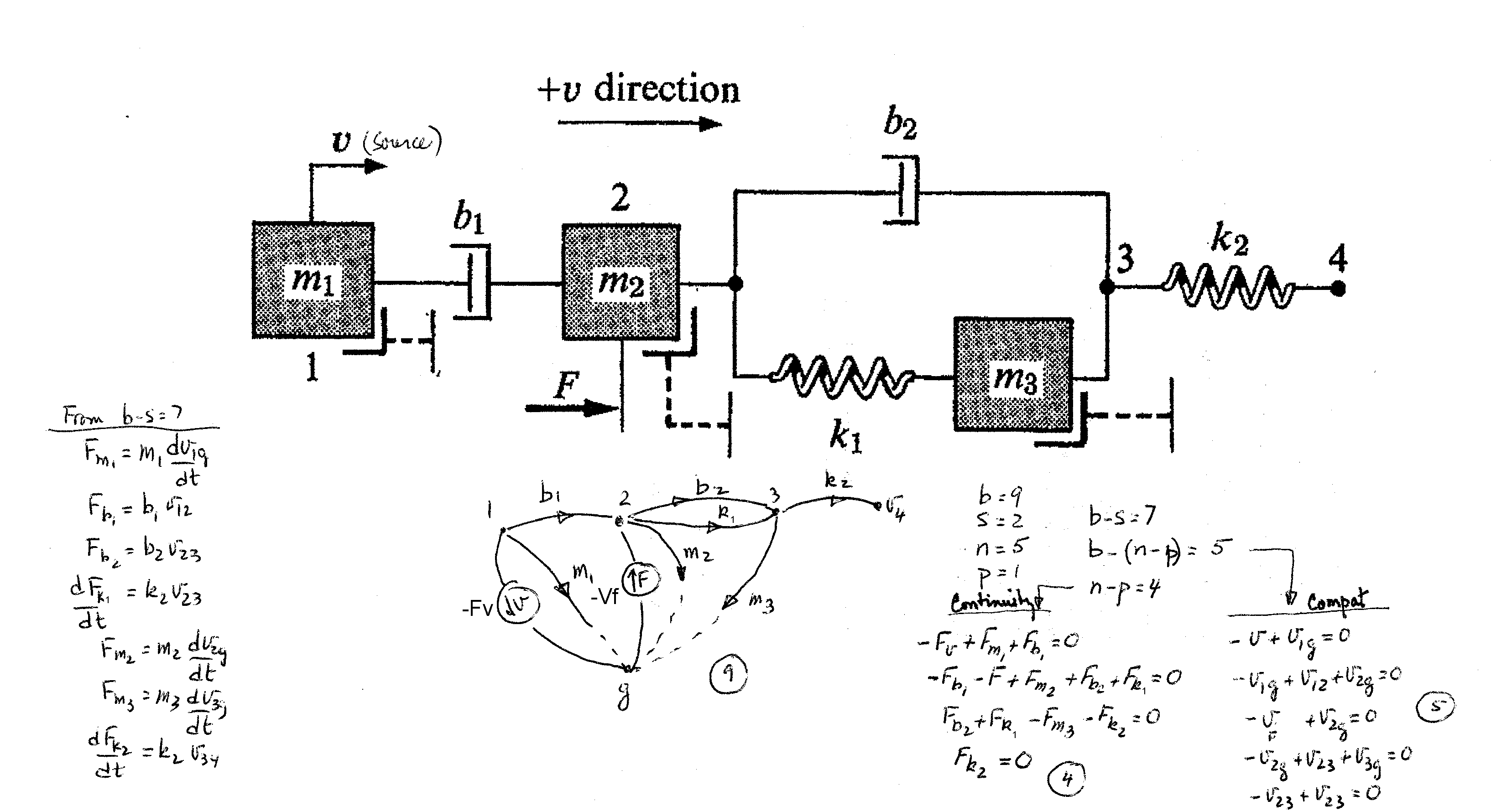
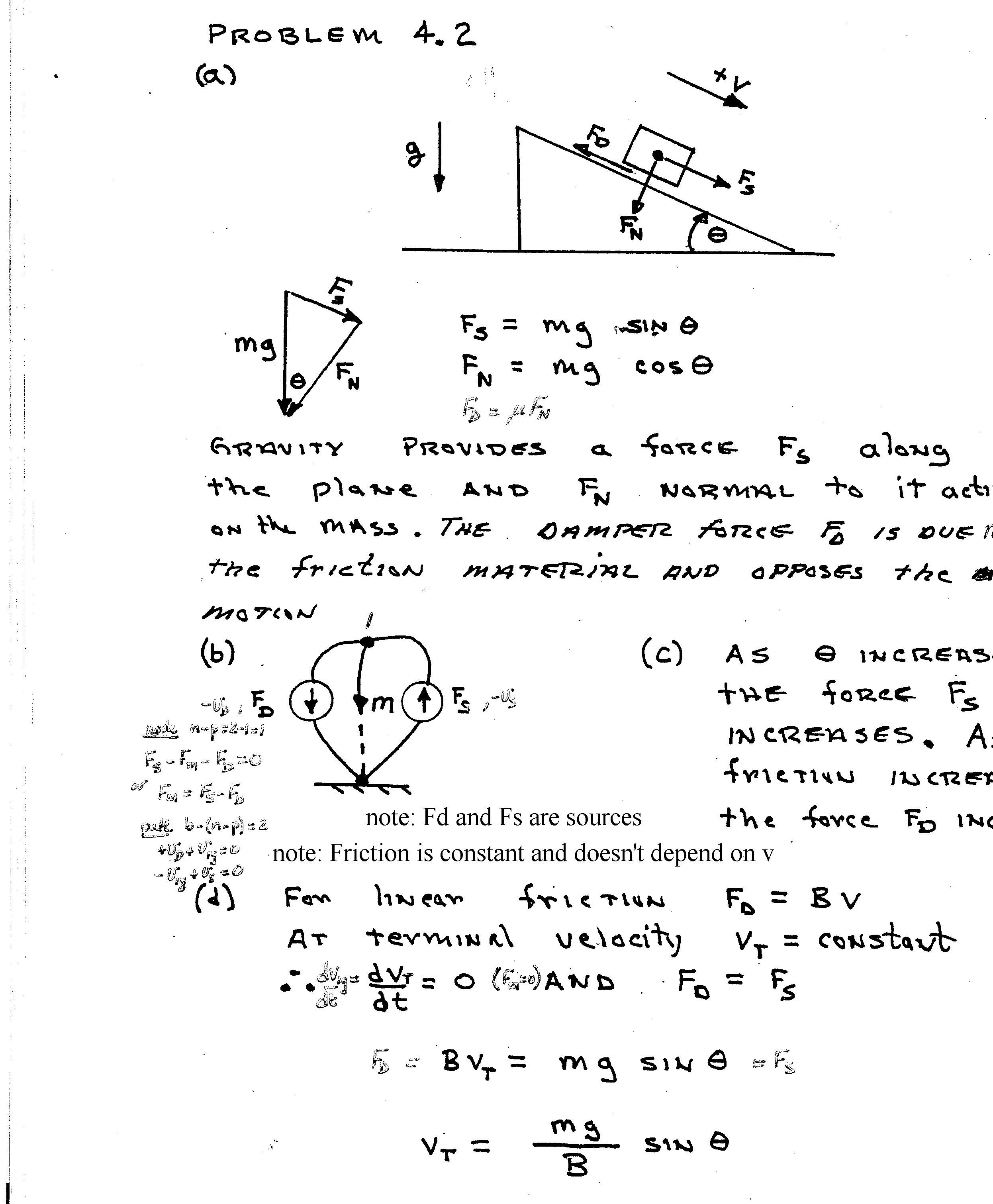
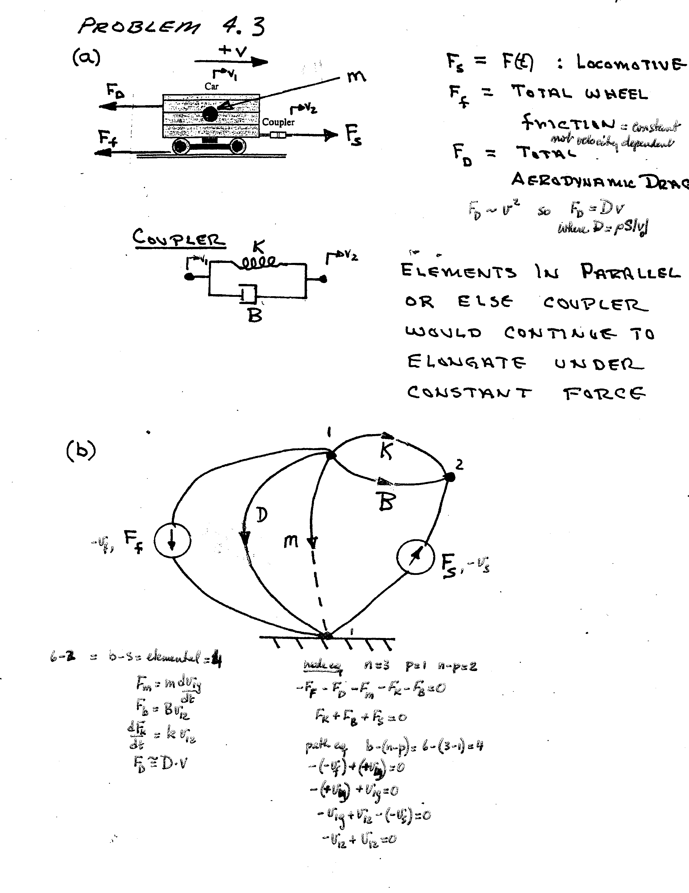
Please do problems 4.1, 4.2, 4.5 and 4.11 in your system dynamics books.

Here is the material that goes with Lecture 12 video: page 54, These are the solution to page 54 top and bottom problems page 55, page 56. We also cover page 57, page 58,

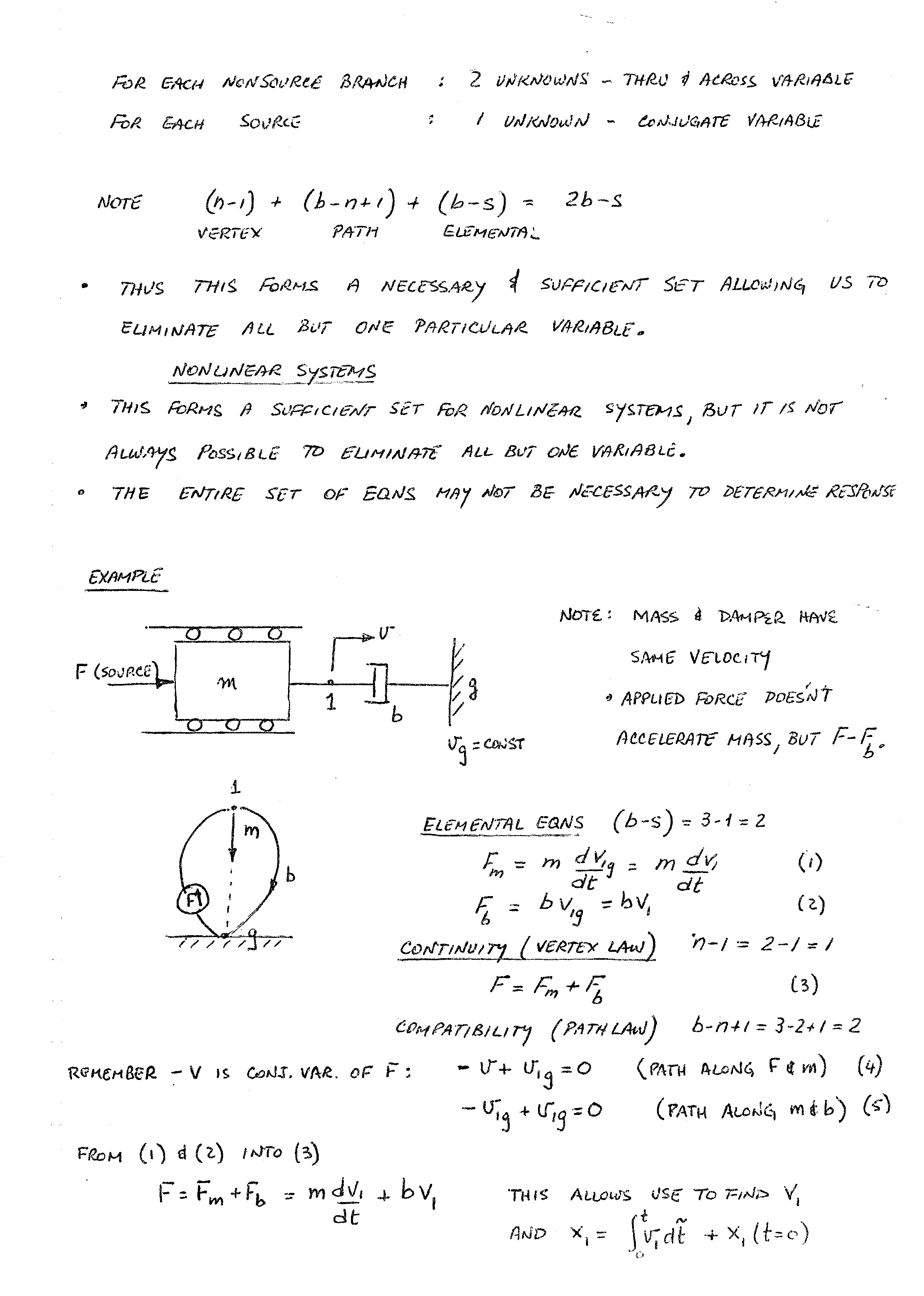
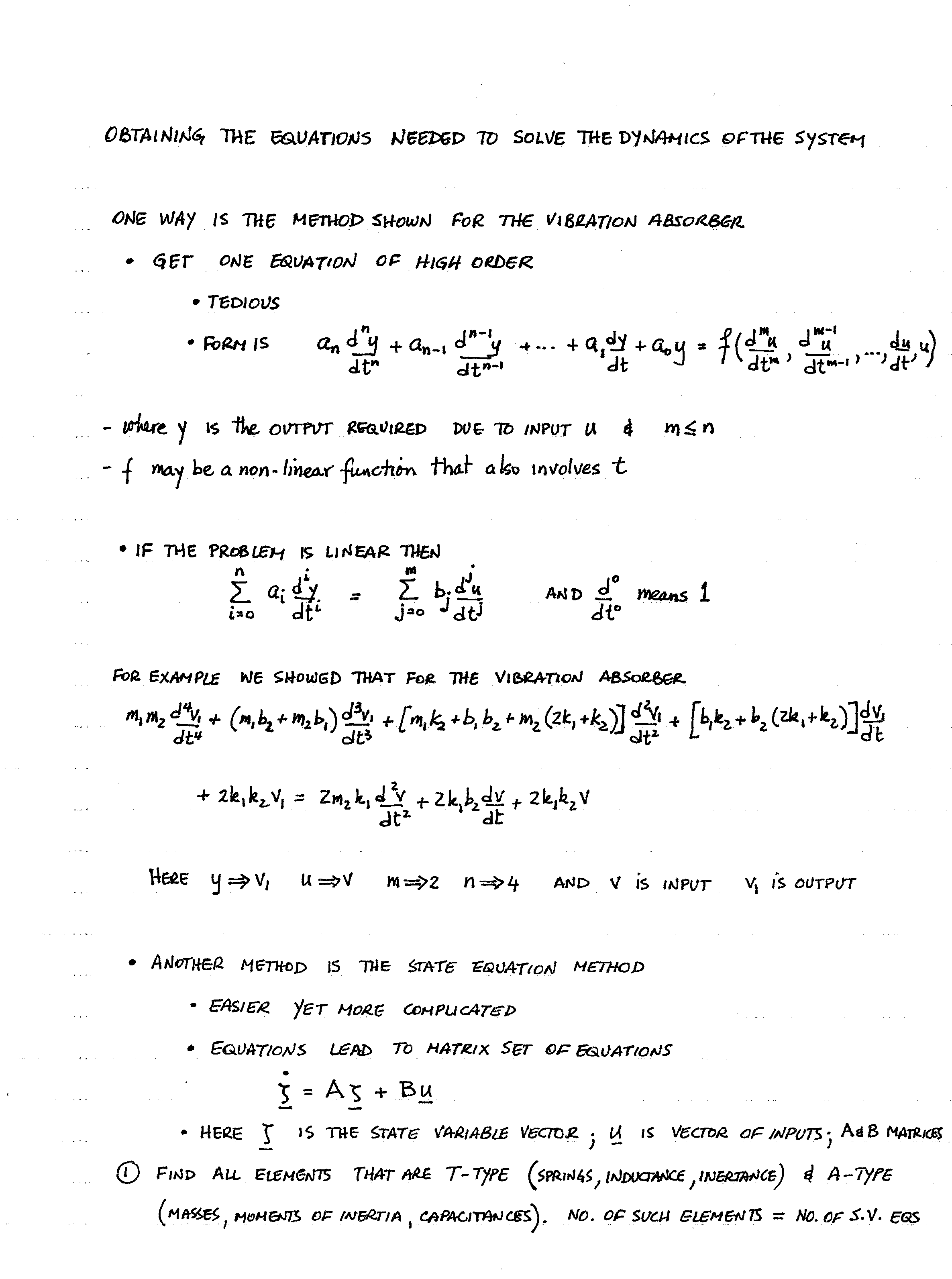
We now begin talking about state equations.

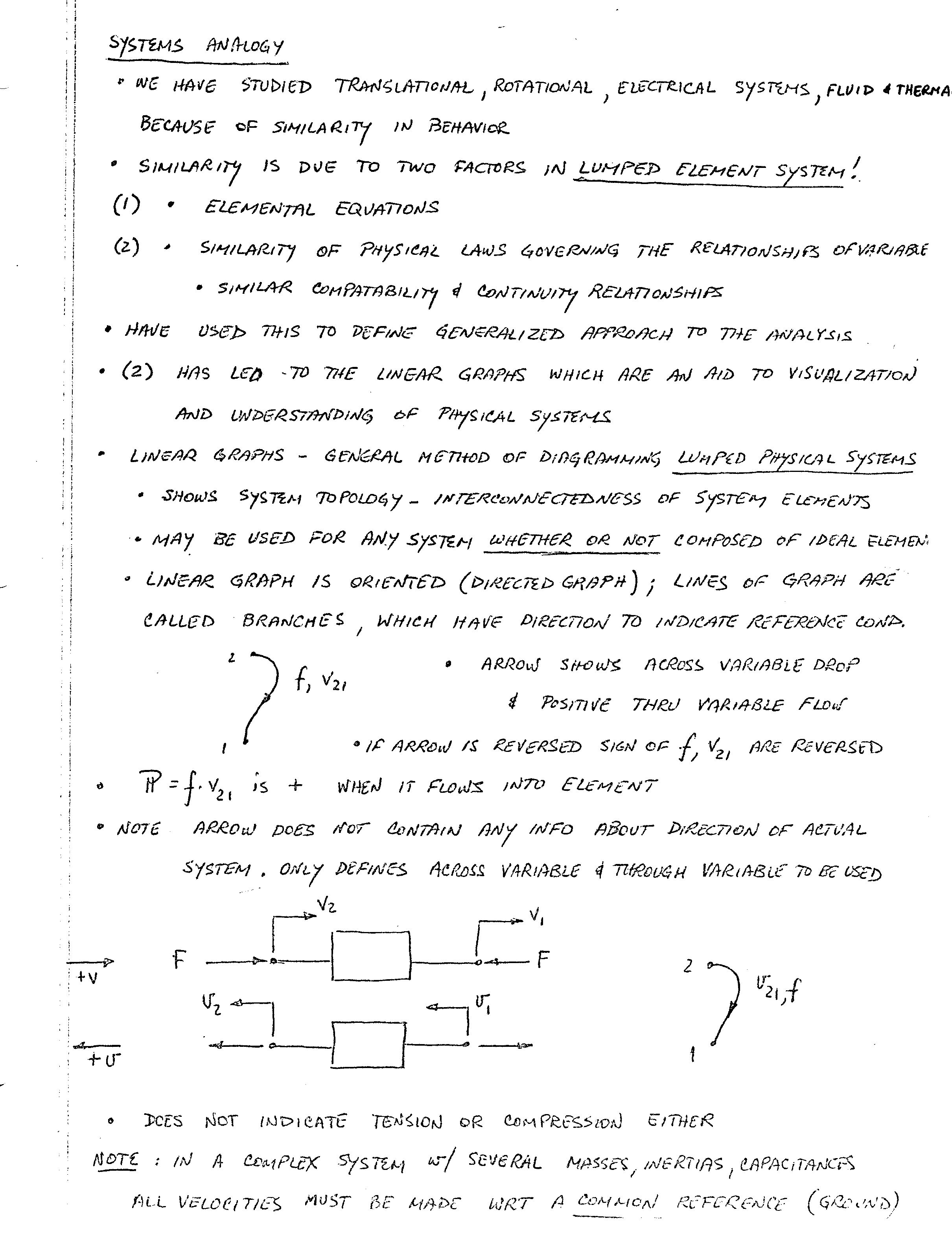
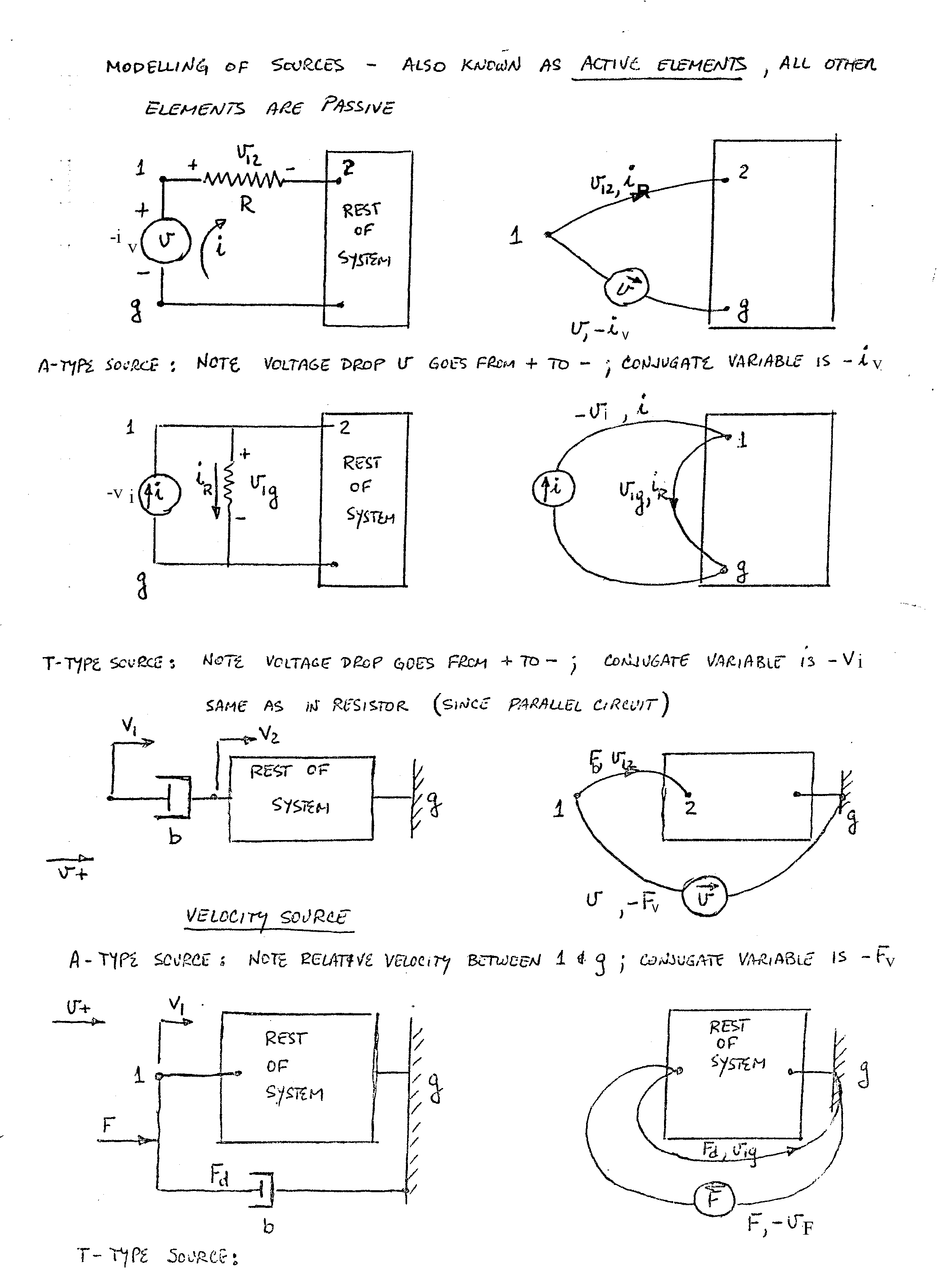
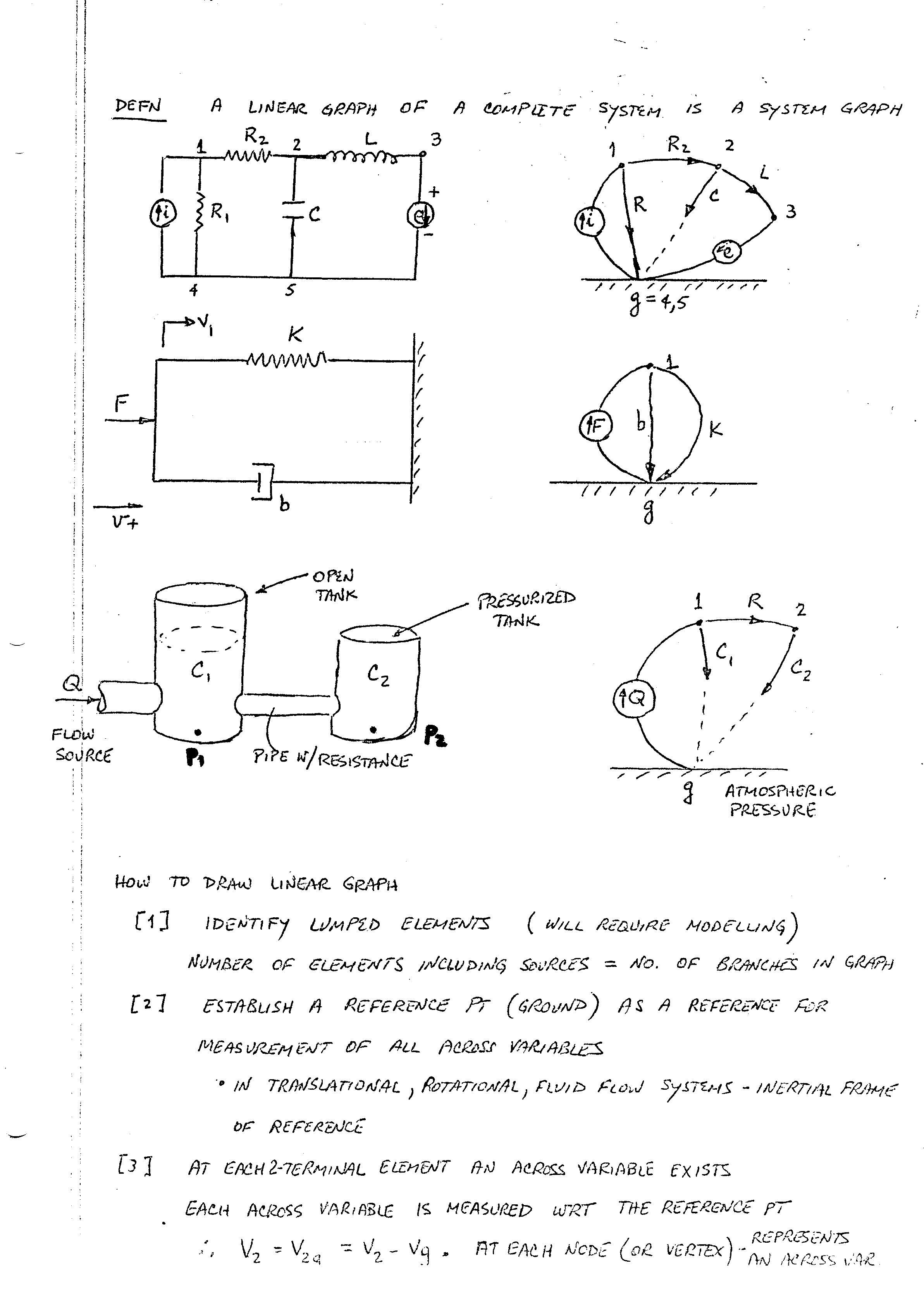
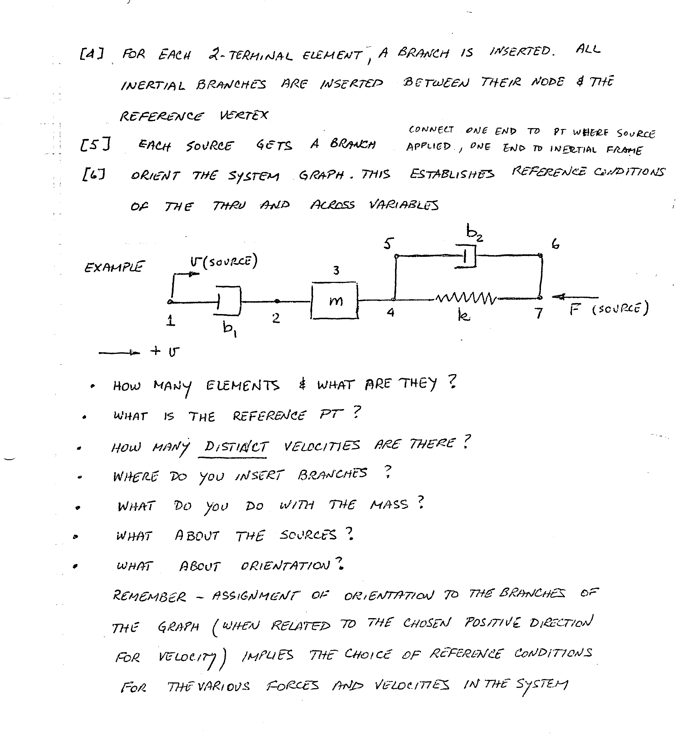
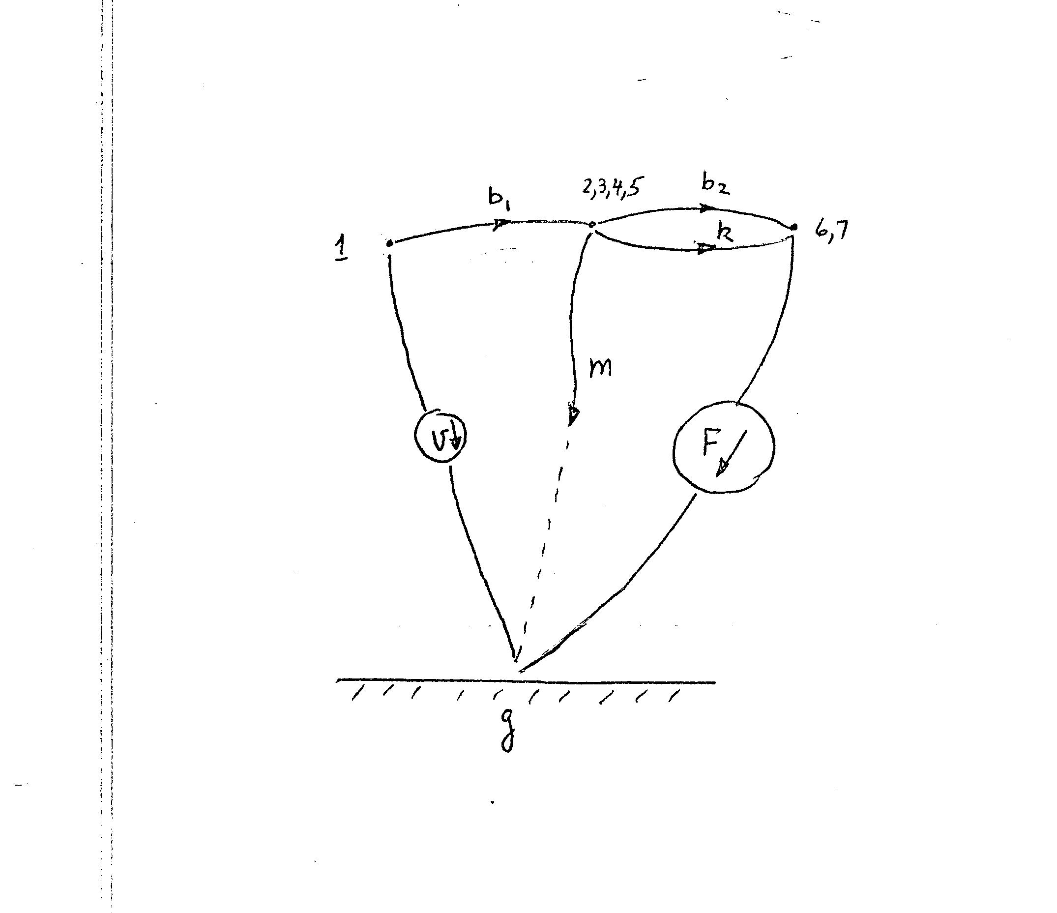
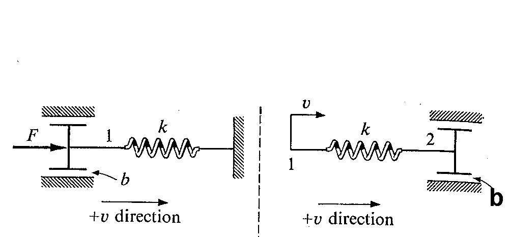
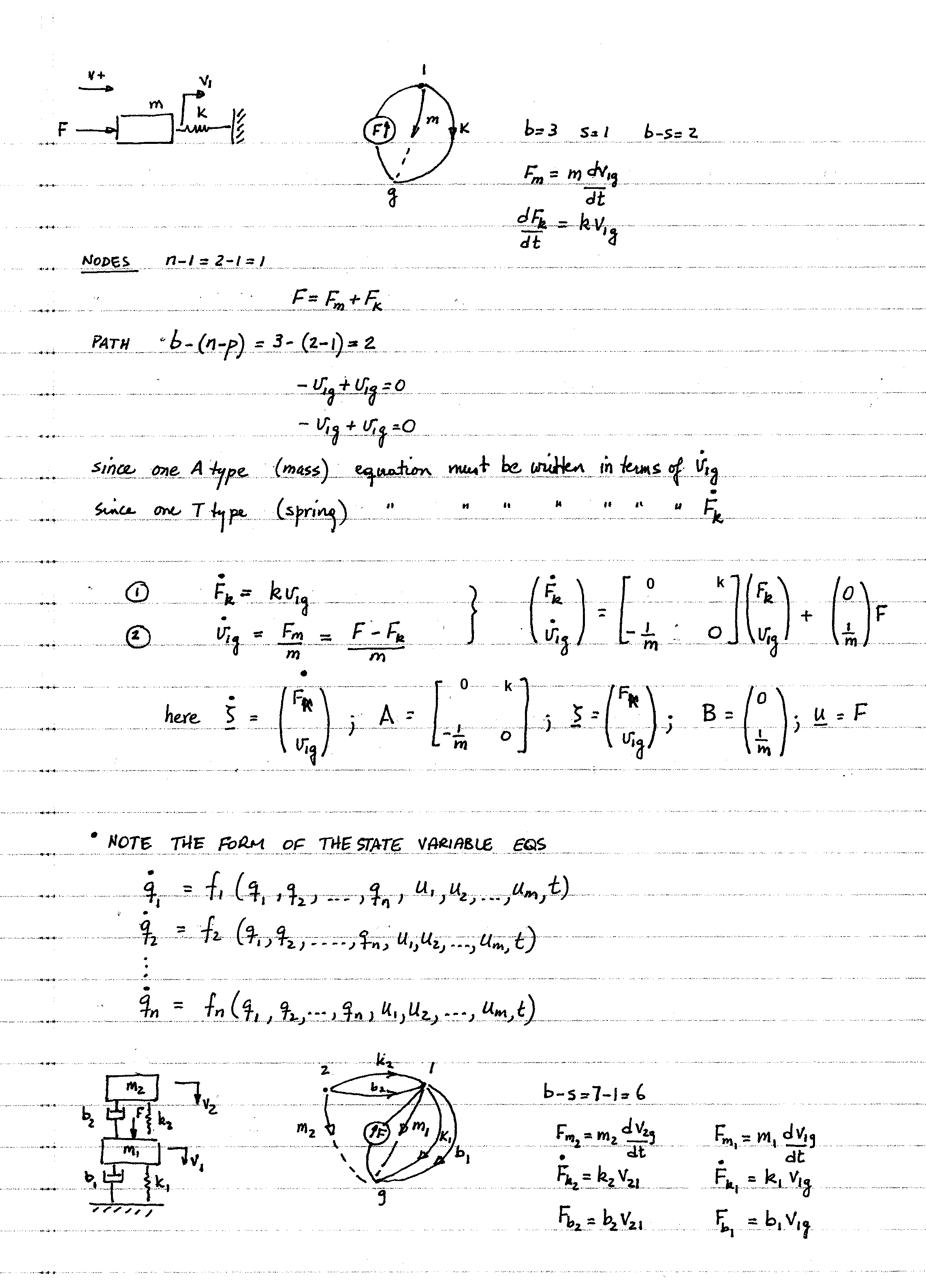
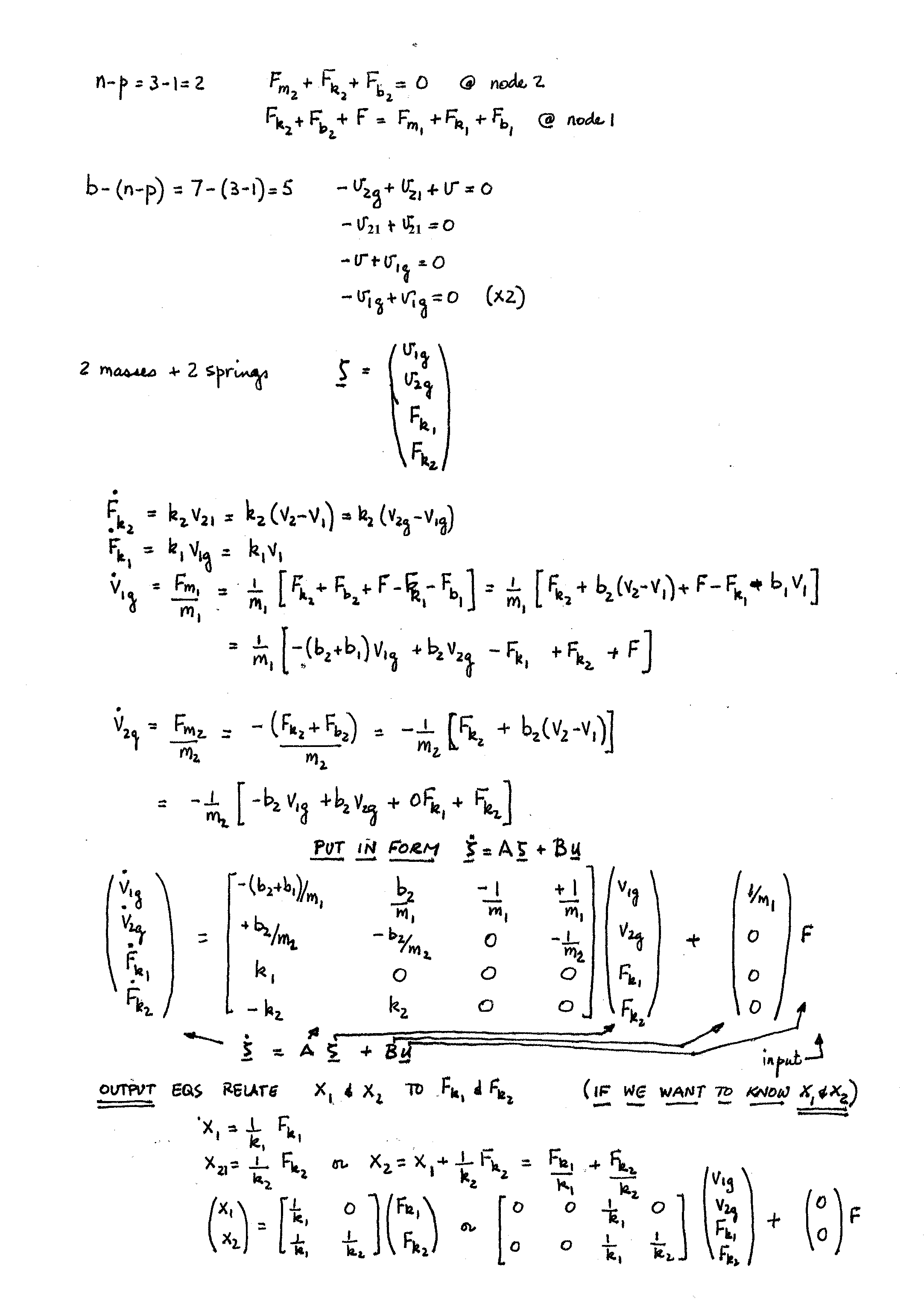
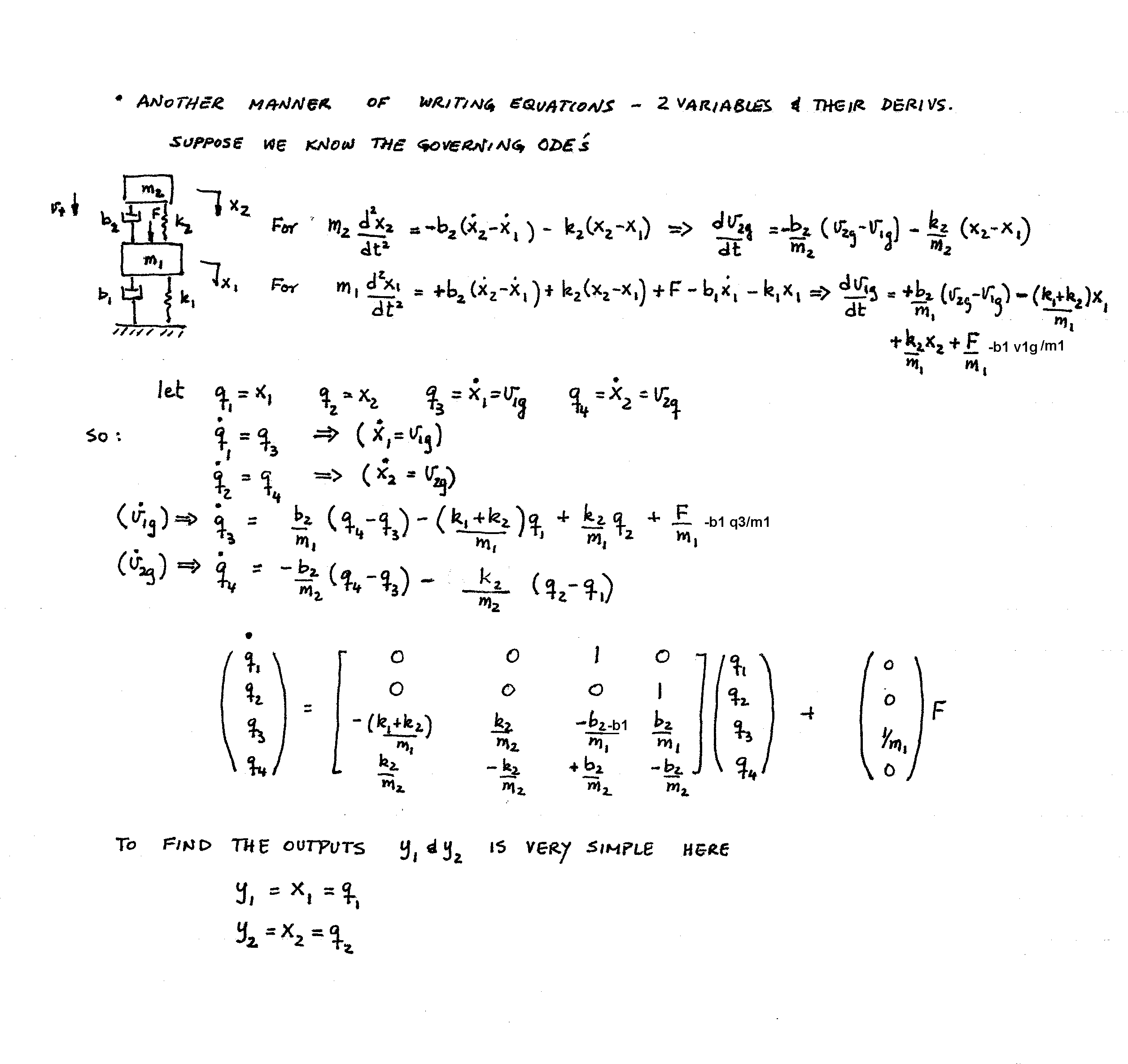
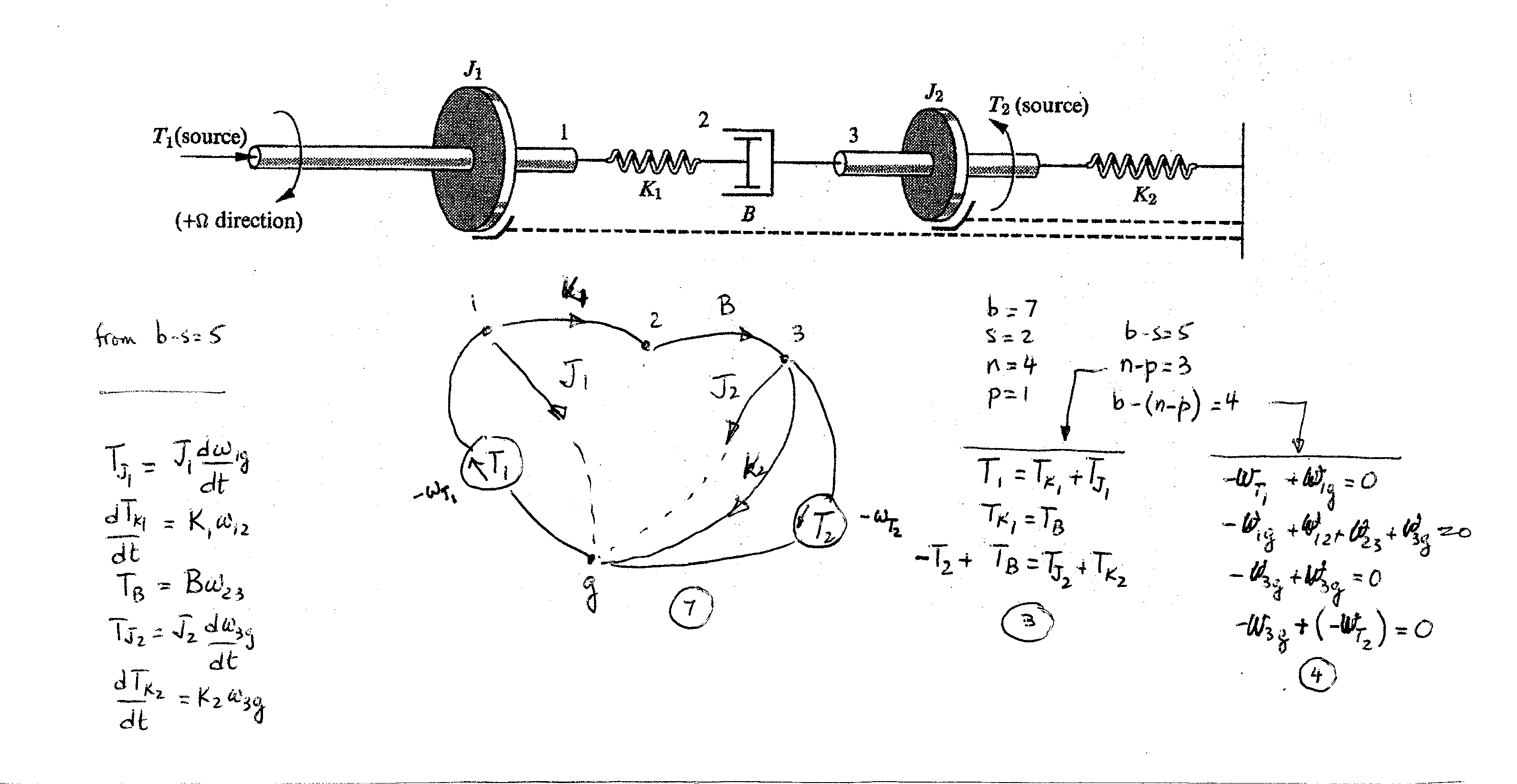
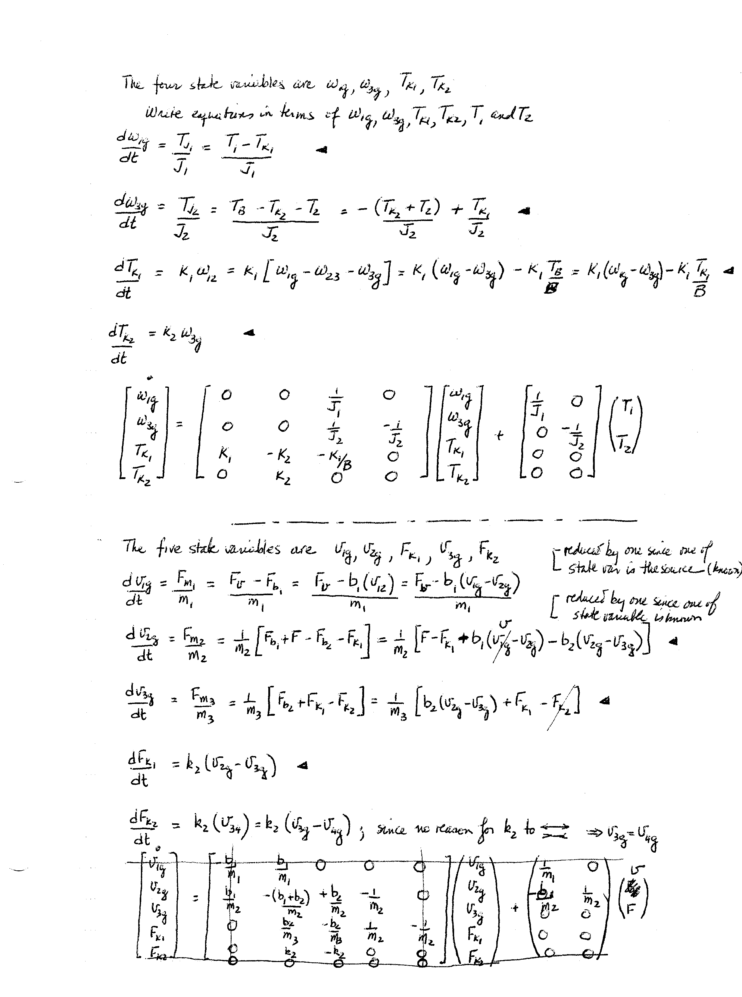
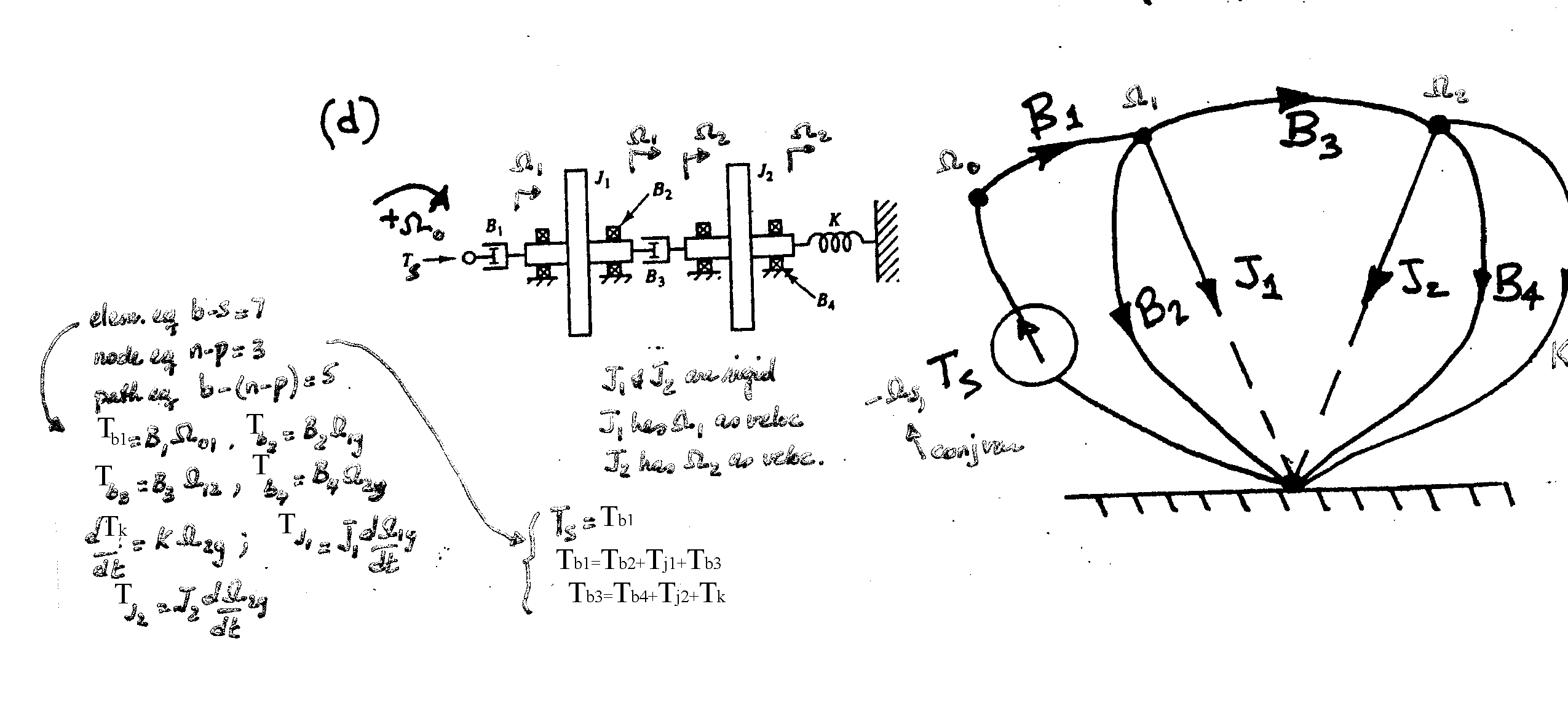
I AM INCLUDING HERE TWO PDF FILES THAT MIGHT HELP YOU: ONE IS ON LINEAR GRAPHS AND ONE IS ON STATE EQUATIONS. THESE DOCUMENTS ARE THE PRECURSOR DOCUMENTS THAT LED TO THE BOOK SYSTEM DYNAMICS, AN INTRODUCTION, BY ROWELL AND WORMLEY. You can find more examples for deriving state equations. Please note that the figure numbers used in the file can be found at the end of the file.

You are also suggested to develop the state equations for three problems -- the two problems we did (given on page 54, 55 and 56 of the notes on the website) and problem 6.15 in your book.

We now begin talking about state equation solutions. This solution methodology depends on understanding matrices. For those who need a review of matrices, here it is.

Here is the material that goes with Lecture 13 video: discussed state variables and how to get the state variable equations and how to solve state variable equations- page 57, page 58, page 59, page 60,

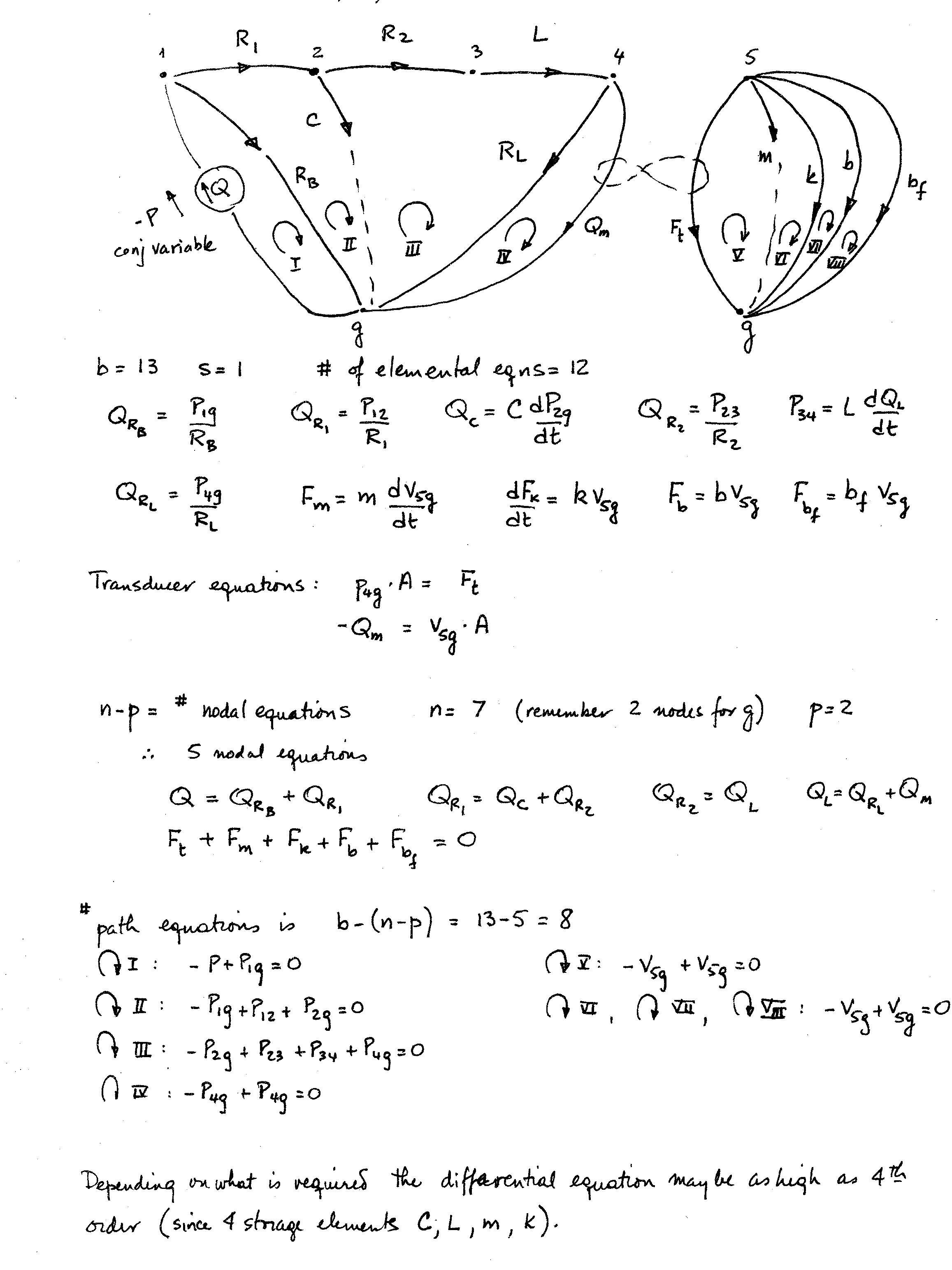
As a review of system graph and state equation derivations we look at this problem. We also show the state equation solution which is given in the top half of the page.

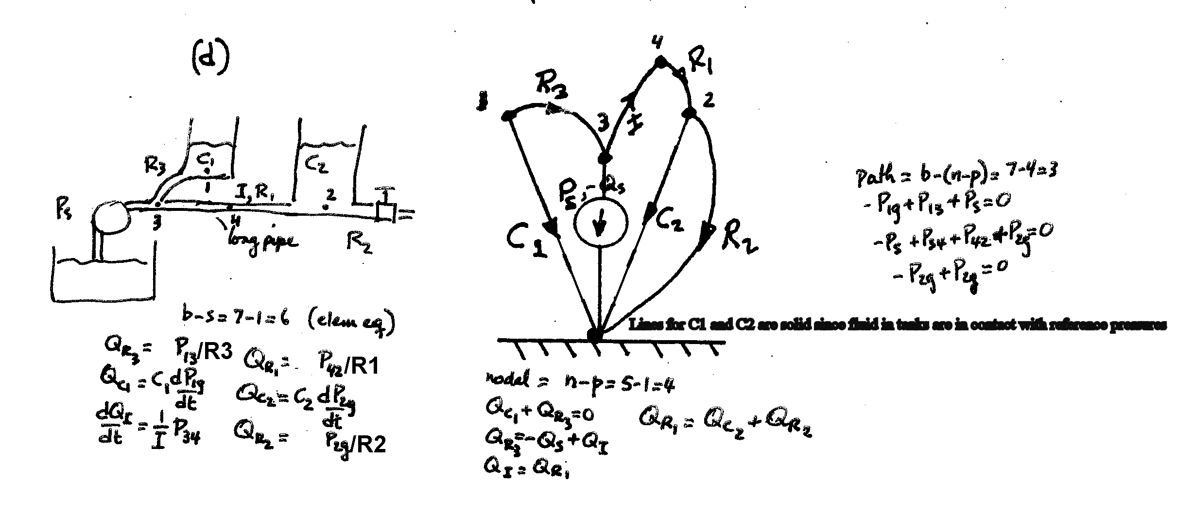
Here is the material that goes with Lecture 14 video: We discuss the following system including getting the system graph. We also show the state equation solution which is given in the bottom half of the page. We have given a handout for the system graph for a fluid system connected to a piston/spring. We will derive the state equations. Also, prob. 7.29 on that sheet will be discussed and one of the state equations will be derived but you are to derive the remaining state equations.

Please note that the first major exam will be on October 24. In the exam you will be given a system and you will be asked to obtain the system graph and to derive the elemental equations (including transformer/transducer equations if any), the node equations (continuity), the path equations (loop, compatibility), and also some if not all the state equations (which are being covered now after system graphs are completed). Formula sheets will be allowed and will be discussed as we get closer to the exam date.

At present, other examples are being discussed in class that may not appear in the videos. It would be to your benefit to come and see more examples so that you can prepare for the

HERE are the solutions to PROBLEMS 4.2, 4.3, 4.6d and 4.11d

Here is the material that goes with Lecture 14-15 video: Halfway through the video we start discussing the numerical solution of the state variable differential equations given in page 61, page 62. This material will NOT be part of the first exam but may be part of the second exam.

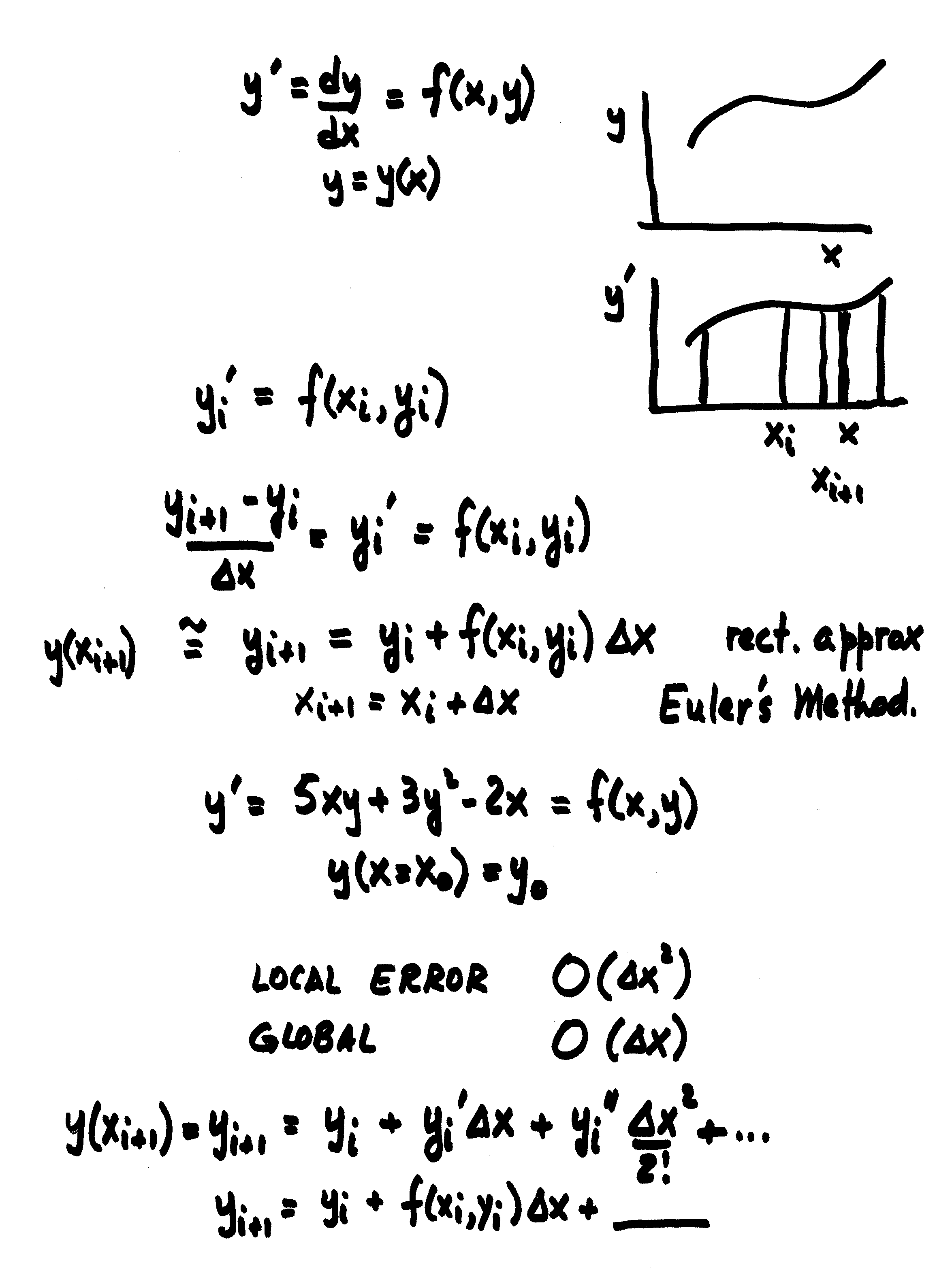
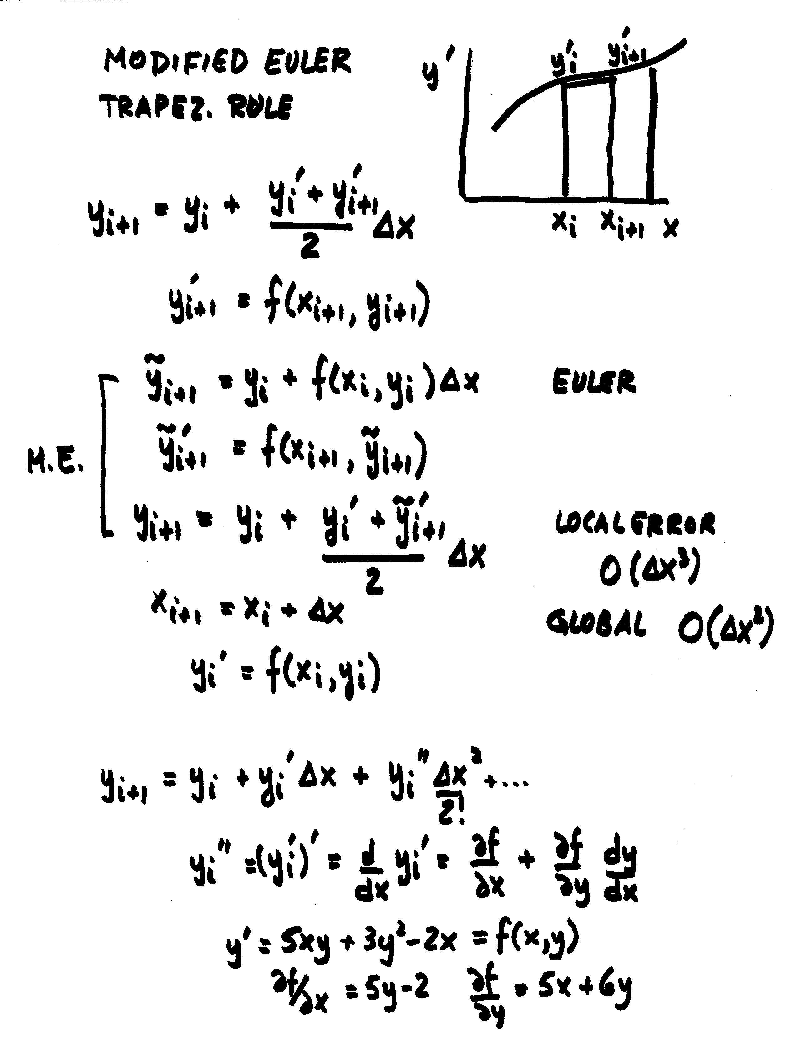
We continue our discussion of numerical solutions of the state equations in Lecture 16. The rest of the numerical solution of sets of first order differential equations will be discussed. A handout will be given in class on the Runge-Kutta method. The handout is from Applied Numerical Methods by James, Wilford and Smith, pages 339-345 and 351-353. We will look at several examples and how they could be used in the different numerical methods discussed, namely: Euler, Modified Euler, Runge-Kutta Second Order method, Runge-Kutta Fourth Order Method

We continue our discussion of numerical solutions of the state equations in Lecture 17. We will work on several problems (4^th order and 2^nd order RK methods).

REMINDER the first MAJOR exam will be on October 24. In the exam you will be given a system and you will be asked to derive the elemental equations (including transformer/transducer equations if any), the node equations (continuity), the path equations (loop, compatibility), and also some if not all the state equations (which will be covered shortly after system graphs are completed). you are allowed 3 8.5 x11 in formula sheets (back and front). You can put pgs 171-172 of your book, the 4 tables (3.1-3.4) and notes to yourself. NO SOLVED PROBLEMS ON THE SHEETS, OTHERWISE YOUR SHEETS WILL BE CONFISCATED.

you are allowed pens, pencils, erasers, straight edge and your simple calculator, if needed.

Turn OFF all cellphones and electronic devices. Your phones cannot be used as calculators.

We begin the vibrations portion of the course. Here is Lecture 18 video: equation of motion for linear mechanical, linear rotational, inverted pendulum

Lecture 19: 2^nd examination on system graphs. We continue with the vibration of undamped SDOF systems

Here is Lecture 20 video: equivalent springs both linear and rotational, springs in parallel and series

Please start reading the first and second section-Chapter 1 and 2 materials from the materials obtained from the office manager (EC3475). I will be assigning examples out of those materials. So it would be to your benefit to come pick up the copies for your group.

Third Exam (2^nd major exam) on numerical methods is announced for Nov. 6, 2019 (THIS IS A CORRECTION). The exam will cover numerical methods. See next page for details.

Out of the photocopies of the first two selections do the following: Problems 1.7 to 1.10, 1.13, 1.16, 1.19, 1.22, 1.26, 1.27, 1.29, 1.31, 1.32, and 1.36. Solutions will be posted in a week’s time.

Please make sure that you have the following information about second order systems, namely:

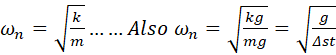where g is the acceleration of gravity and D_stis the static displacement of the system; that is, weight of the system = k*D_st.

Please use the Greek capital letter D for the static displacement instead of the normal d, as the letter d is to be used for the logarithmic decrement, and they should not be confused.

And for systems with damping included: =2ςω_n and =ς and Ccrit=2√mk =2mω_n =2k/ω_n

Lecture 21: 2nd examination is announced for Wednesday, Nov 6 (THIS IS A CORRECTION) and will be on numerical methods. It will cover the numerical solution of state equations. You will be allowed pens, pencils, straight edge, erasers and your calculator. You will be allowed three 8.5 x 11 formula sheets. Please ensure your formula sheets include the formulas for the Euler, Modified Euler, Runge Kutta 2^nd order, Runge Kutta 2^nd order Midpoint, 4^th order Runge Kutta and how to handle numerically the solution of one or more state variable equations.

In addition you should know the local and global errors for each of the methods. You should know how to use that information to show the advantages of one method over another as we did in class, i.e., comparing global errors between different methods to find the stepsize, or to determine the number of floating point operations saved for a certain number of steps.

Any solutions found on your formula sheets will have the formula sheets confiscated.

Here is Lecture 22 video: equivalent springs and masses using equivalent potential and kinetic energies

Please review the videos for Lessons 18, 20, 22 as we will be doing similar type problems for you to understand the method of solution.

Here is Lecture 23 video: we look at damped systems, derive equations and talk about overdamped, critically damped and underdamped systems

Please note that for underdamped systems: the logarithmic decrement, δ, equals where ζ is the damping ratio, C/Crit.

Also we show that δ = (1/N) * ln(x_o/x_N) = (1/N) * ln(x_i/x_i+N)

where N = the number of cycles between the first and last measurement. x here is the displacement and the subscript “o” means the first measurement value. The formula also applies between any N cycles, meaning starting from cycle i and going to cycle i+N.

We will discuss the forced vibration of systems and cover the topic of resonance.

The following change is announced: Projects will be due on Monday, December 2 at 3pm in my office. Do your best to turn it in physically. If you cannot make it, please contact me for other arrangements.

The following is also announced: Your third major exam on vibrations will be on December 4.

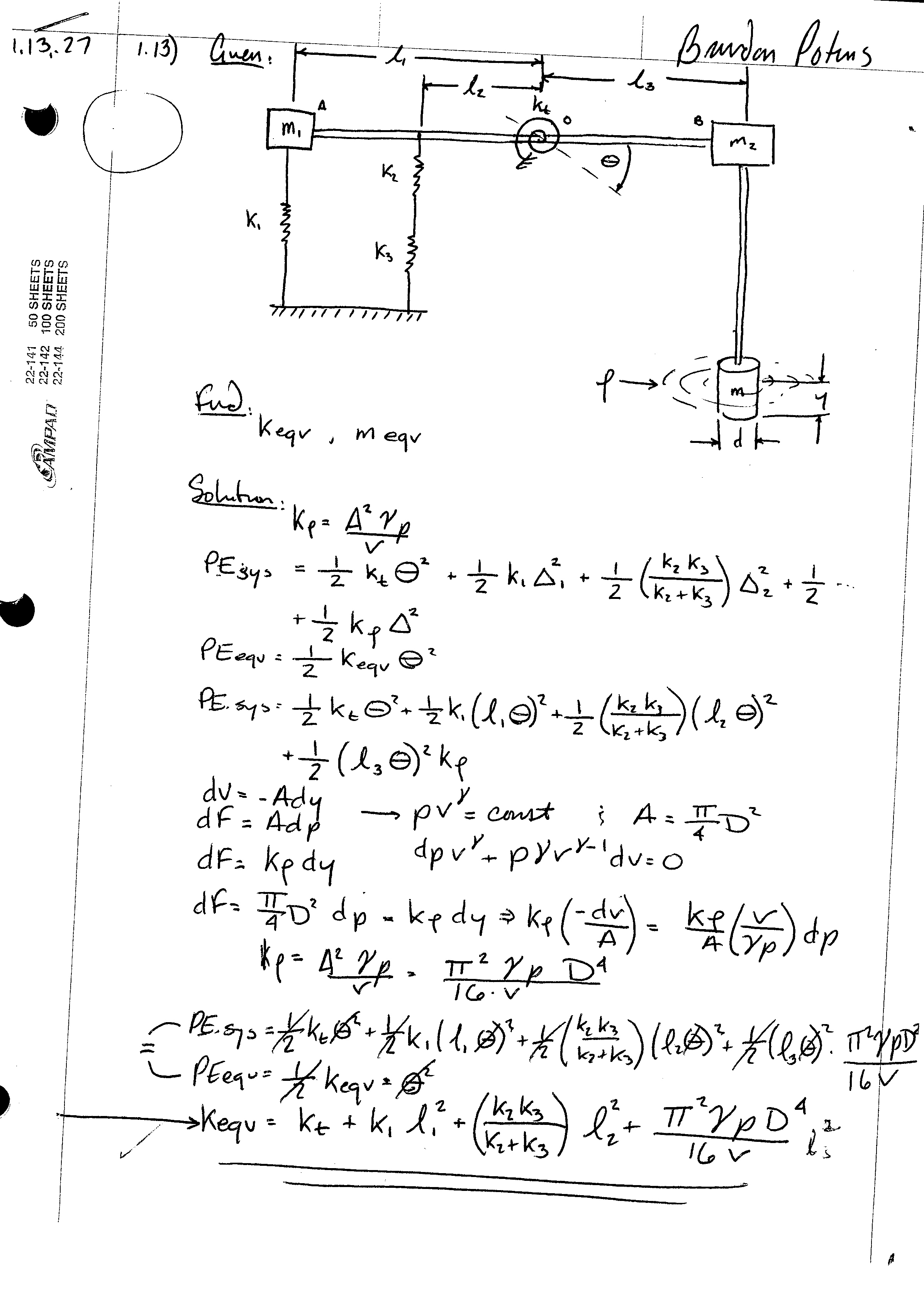
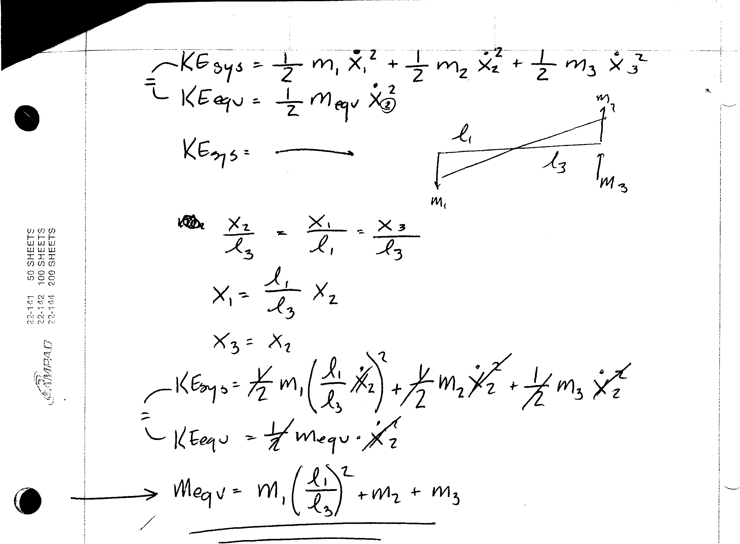
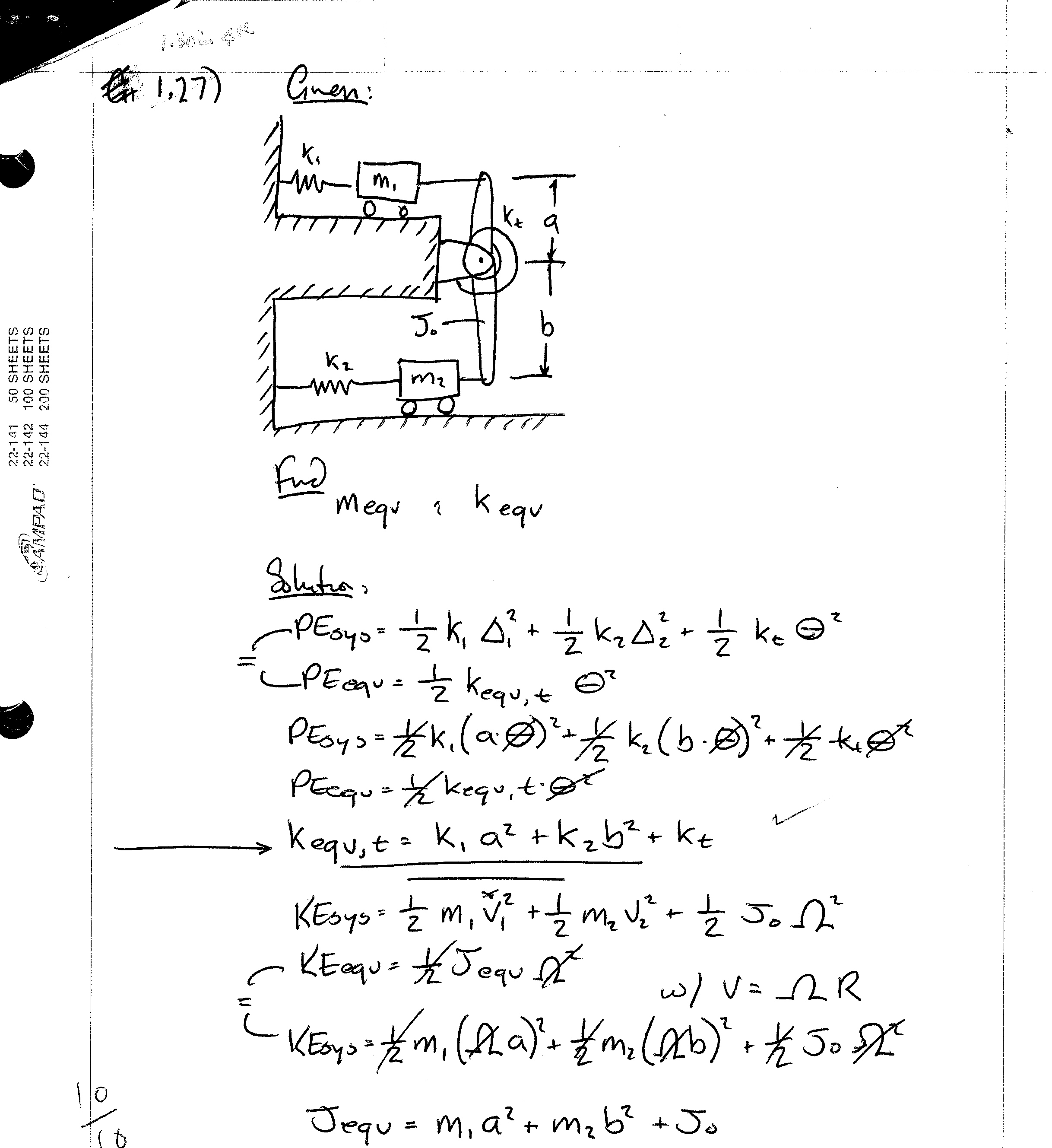
You will be allowed 3 8.5 x11 sheets of formulas. The topic of the exam includes: vibrations of undamped SDOF system; how to determine k equivalent (look at the Cochin handout) and equivalent masses based on where they are placed using equivalent energies; damped vibration systems with coulomb or viscous damping; systems that are overdamped, critically damped and underdamped. Be able to derive equations of motion. Materials from the forced vibration of a single degree of freedom system including, resonance, calculating the steady state motion for a SDOF system and how to determine forces transmitted to the support.

Here are solutions to some of the problems… problems 1-7 and 1-8, 1-9 and 1-10

Here are solutions for problems 1-13a and 1-13b, 1-29, 1-30, 1-35 and 1-35b

Here is Lecture 24 video: we look at underdamped systems, derived logarithmic decrement and talk about two problems.

Look at Problems 2.1-2.4, 2.6, 2.7, 2.17 to 2.19, 2.28, 2.38, 2.45, 2.52, 2.60, 2.80, 2.82, 2.83, and 2.97 in the handouts obtained from the department.

Please make sure that you have the following information about second order systems, namely:

where g is the acceleration of gravity and D_stis the static displacement of the system; that is, weight of the system = k*D_st.

Please use the Greek capital letter D for the static displacement instead of the normal d, as the letter d is to be used for the logarithmic decrement, and they should not be confused.

And for systems with damping included: =2ςω_n and =ς and Ccrit=2√mk =2mω_n =2k/ω_n

Please note that for underdamped systems: the logarithmic decrement, δ, equals ,

where ζ is the damping ratio, C/Ccrit. Also ζ=δ / sqrt(4π²+δ²), which for z <0.3 can be approximated by

Also δ = (1/N) * ln(x_o/x_N) = (1/N) * ln(x_i/x_i+N)

where N = the number of cycles between the first and the N+1^st measurement. Here x is the displacement and the subscript “o” means the initial measurement value. The formula also applies between any N cycles; meaning, starting from cycle i and going to cycle i+N.

Please make sure you review the videos for Lessons 18-24 as they cover the materials for this last exam.

We will discuss the forced vibration of systems and cover the topic of resonance.

Here are solutions for problems similar to 2-4, 2-6 and 2-7 in the vibrations handout obtained from the department office manager. Problem 2-7 requires moving the springs to the location of the mass.

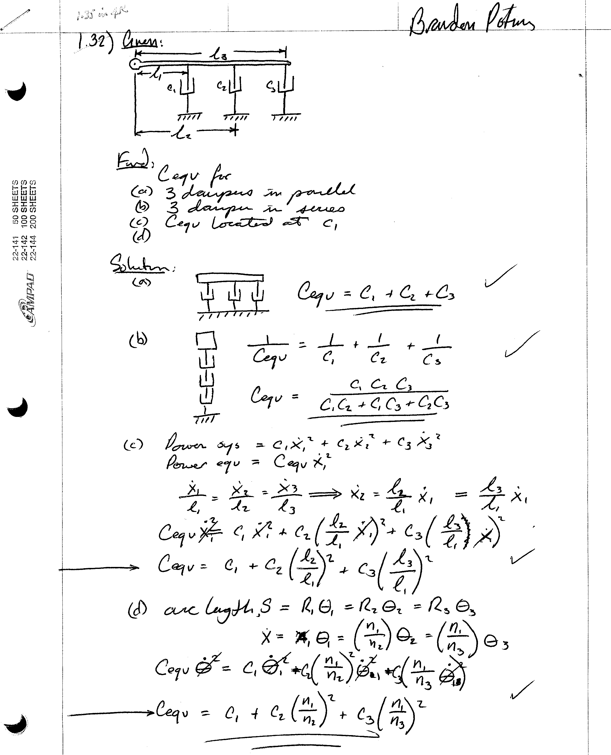
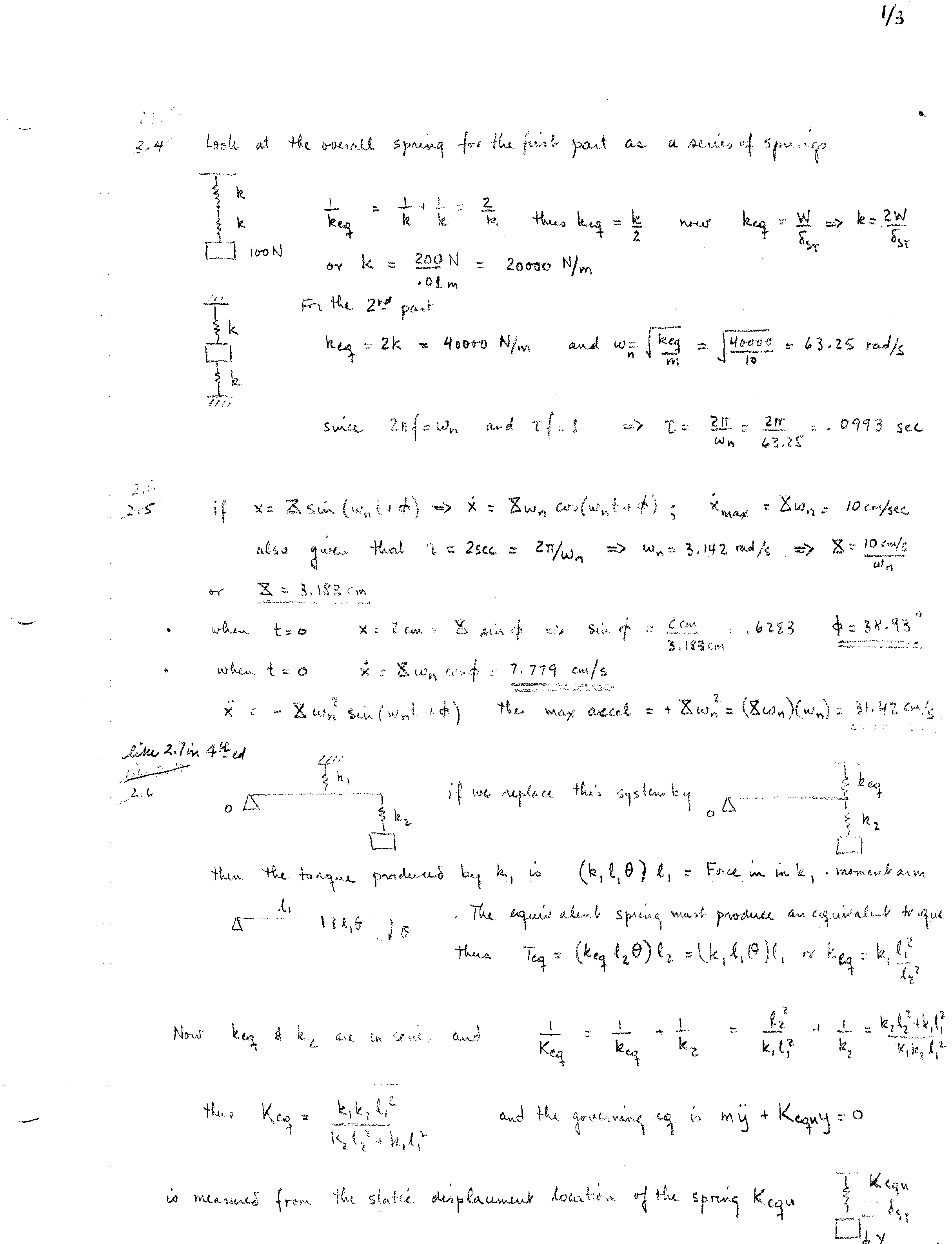
Here are problems 2-17, 2-18, 2-19. In problem 2-17 both springs see the same displacement. For 2-18 use the equivalent k for extension of a wire.

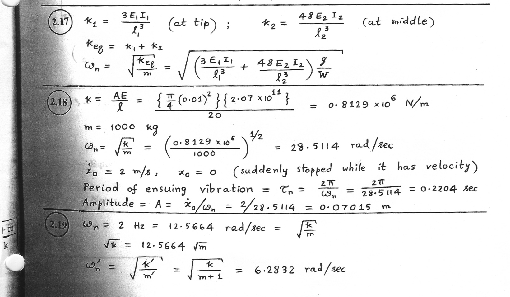
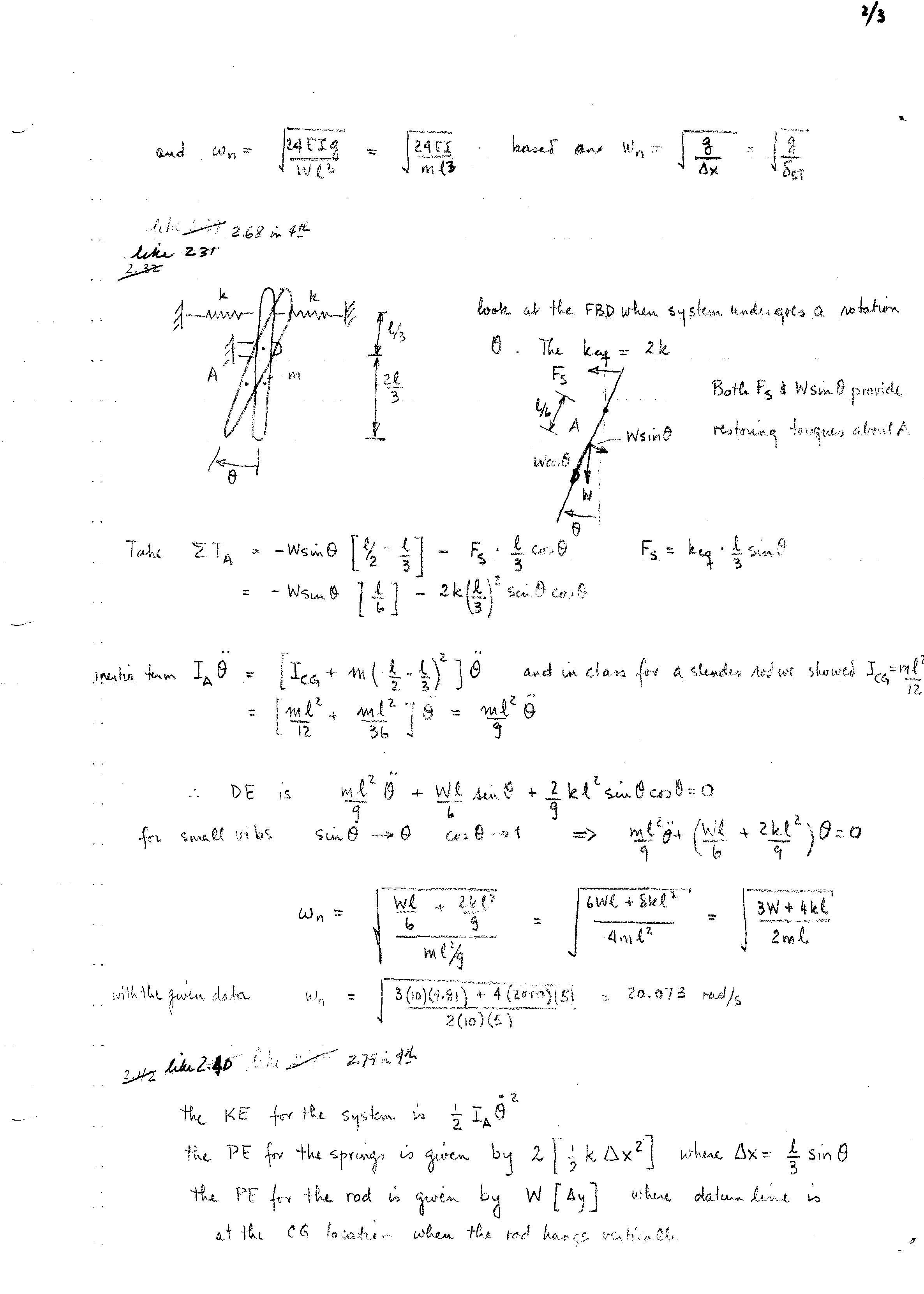
Here are problems like 2-28, 2-38

Here is the rest of 2-38, and problems 2-68, 2-79

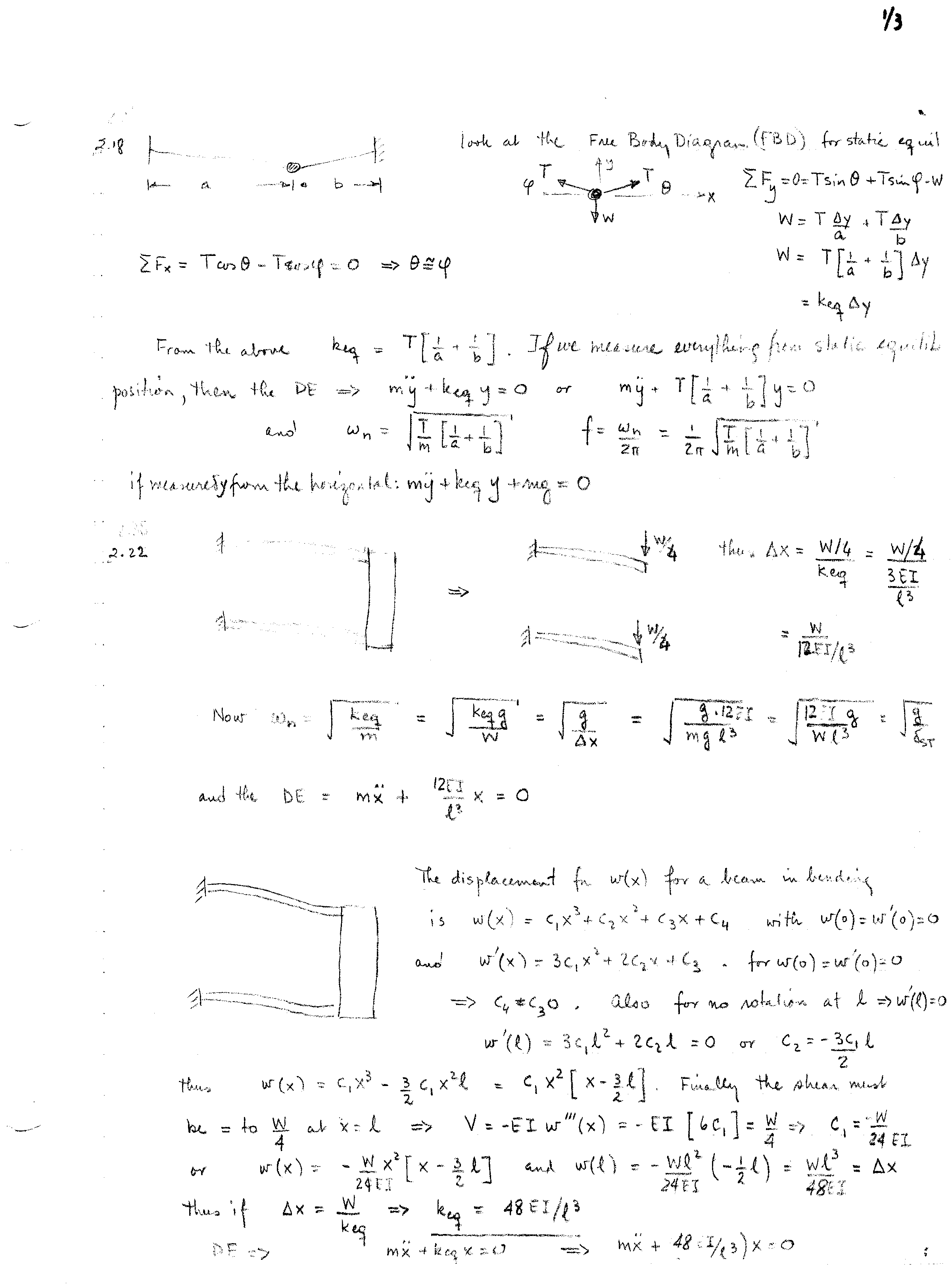
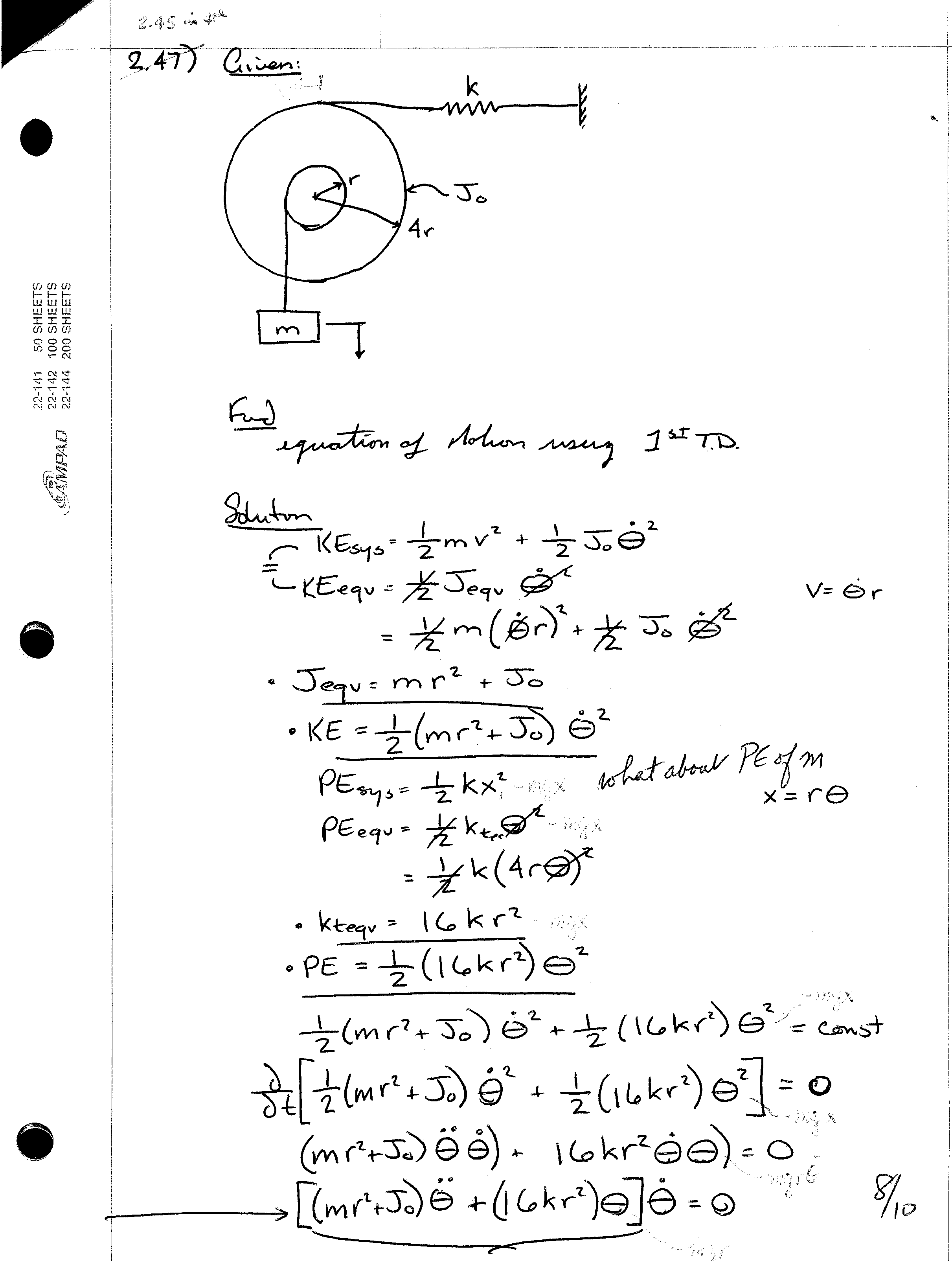
Here is problem 2-45

Here is problem 2-60

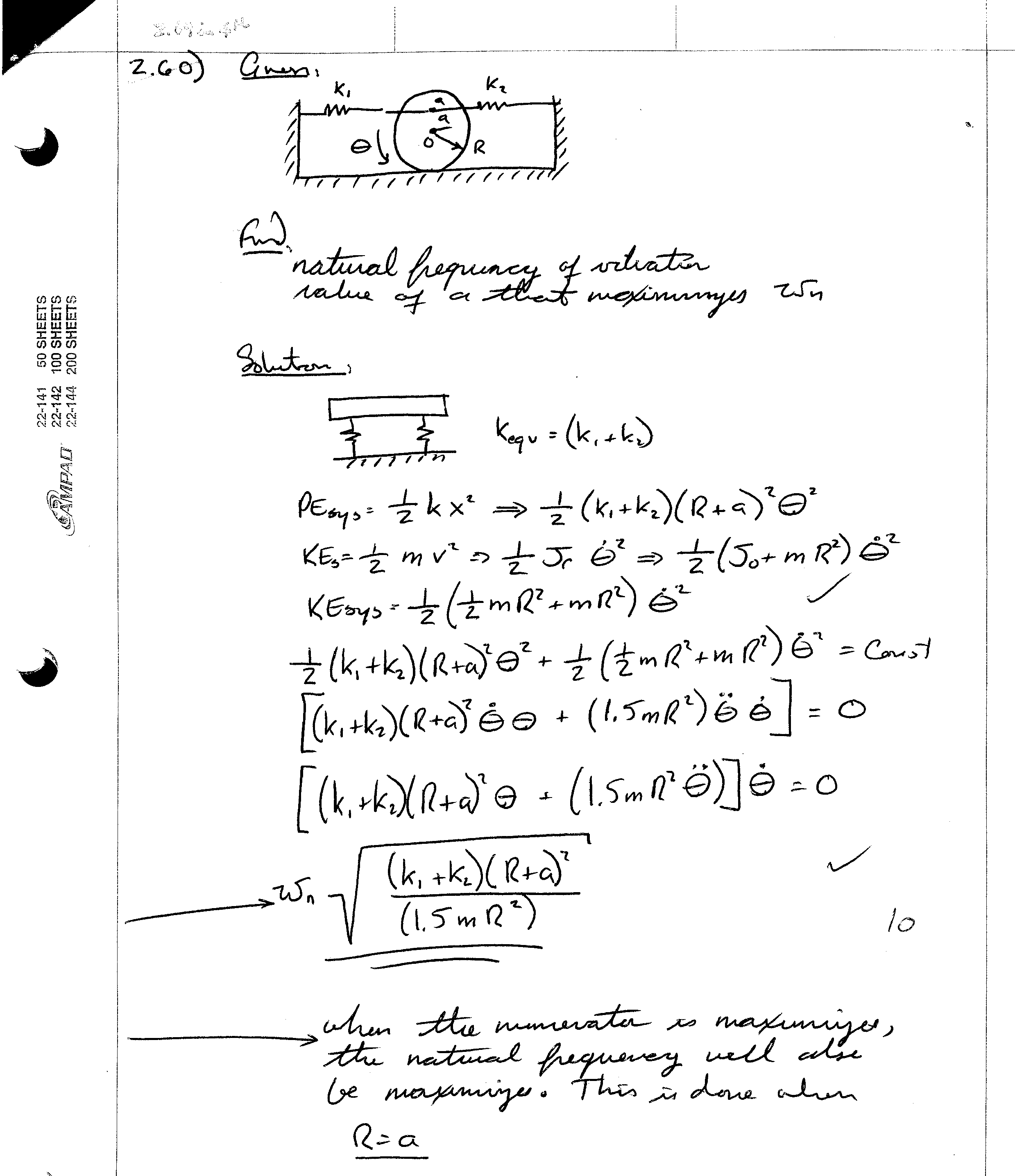
Here, the second problem is like problem 2.80. Note, overshoot represents the maximum displacement above the x=0 line, i.e., when the velocity=0.

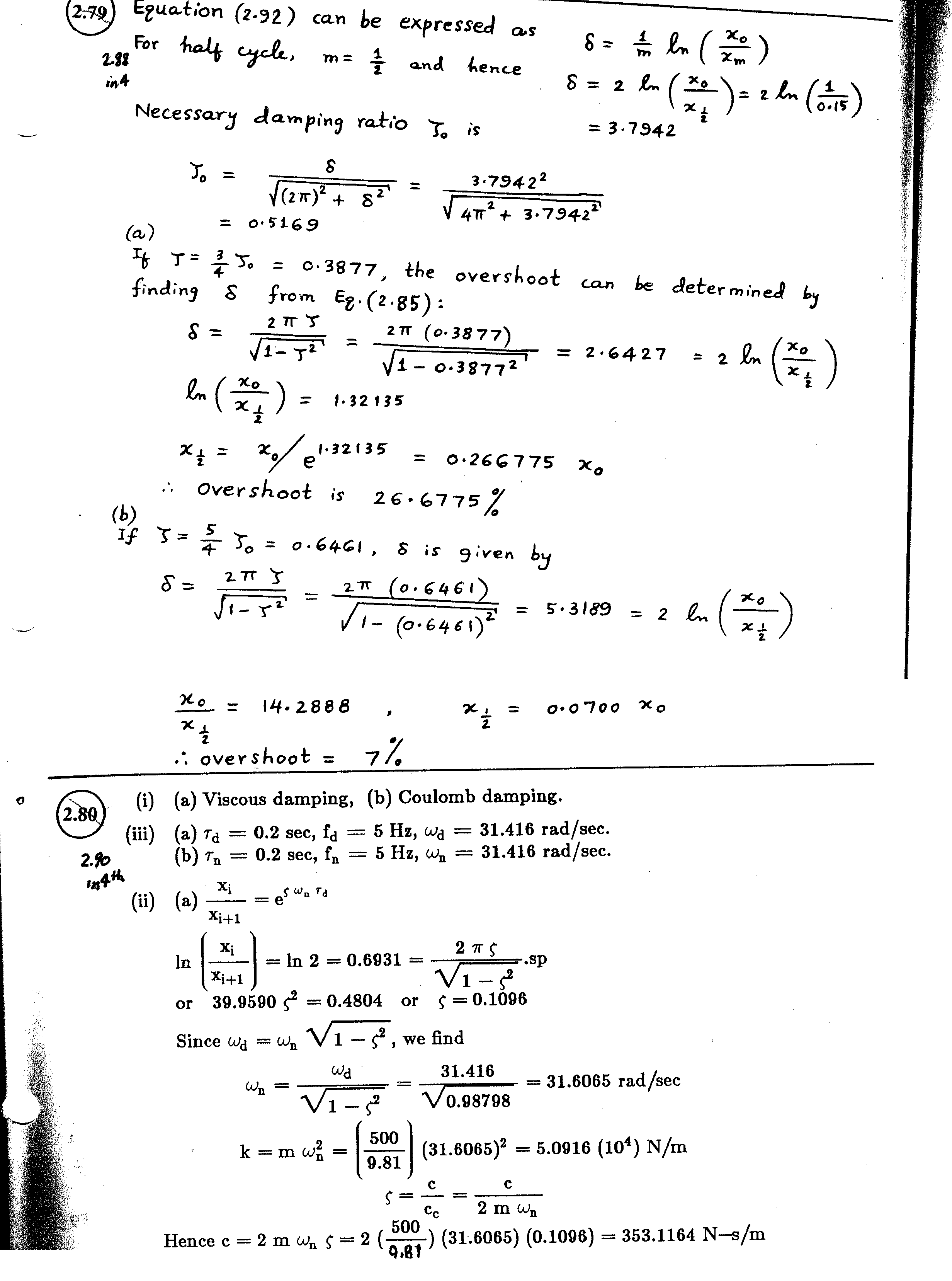
Here are problems the first two are like 2.83, 2.97

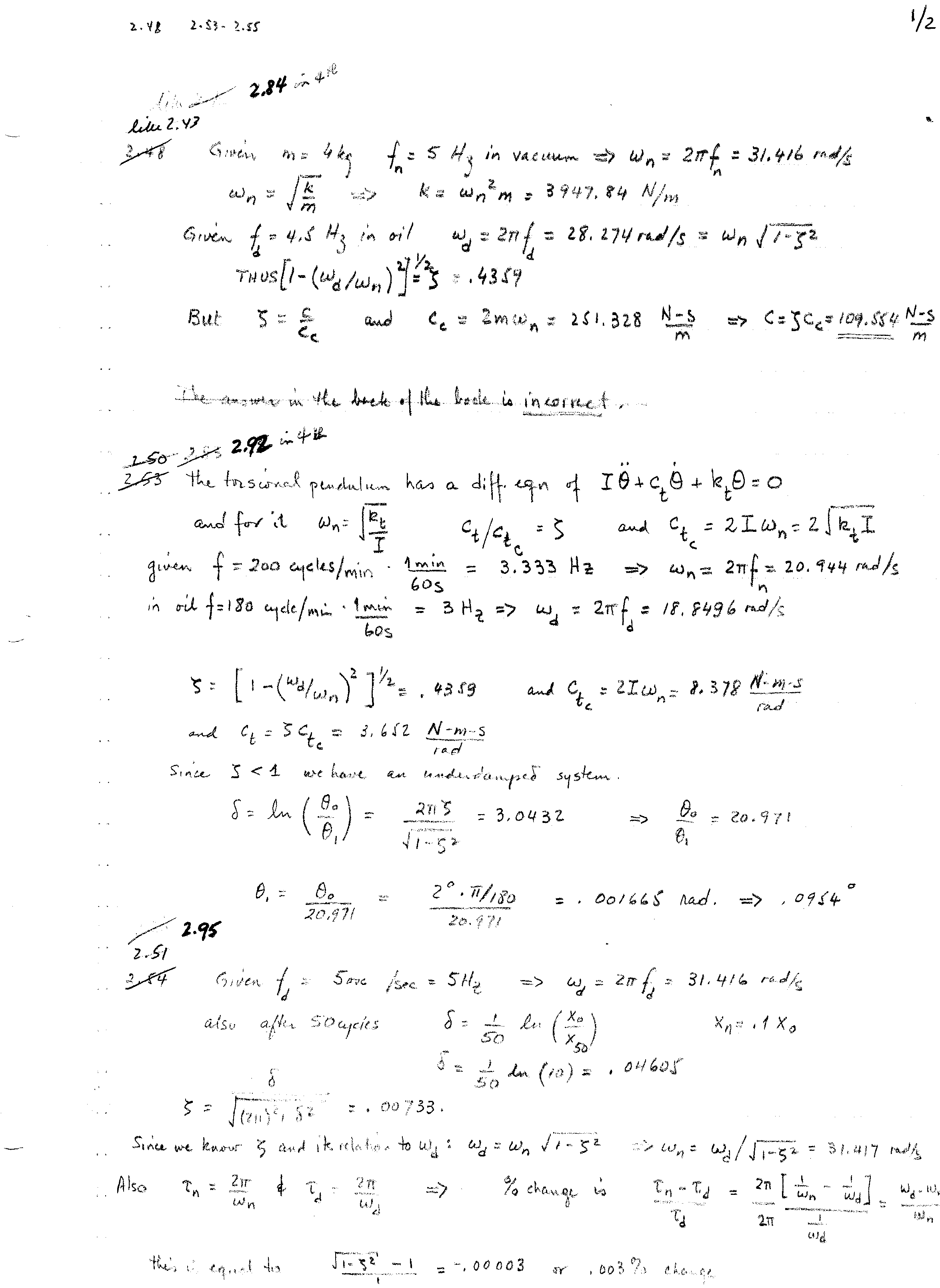
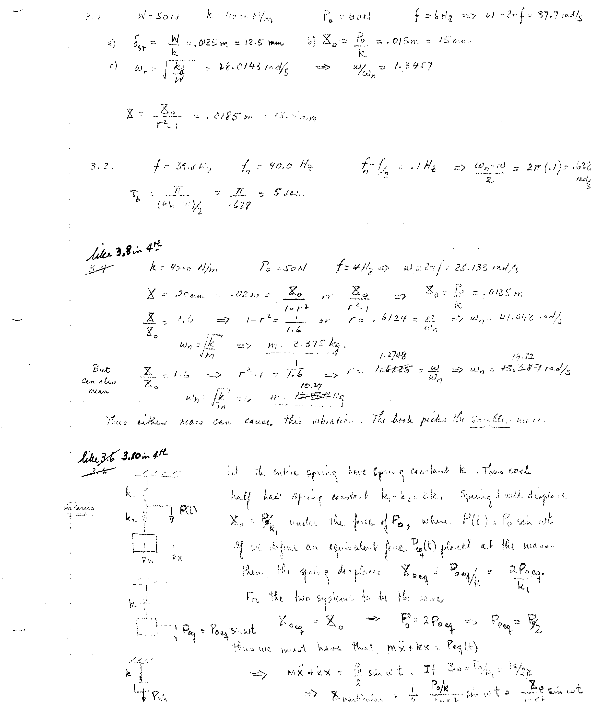
Lecture 25: We begin by discussing the case of forced vibrations. The following problems deal with forced vibrations from Chapter 3 of the handouts obtained from the department office manager. Here are problems 3.1, 3.2, 3.8, 3.10. Also try problems 3.25, 3.26—No solutions will be given for these…

Here is a video related to beats, undamped forced motion

Lecture 27: we start discussion of the rotating unbalance situation and show that the equation of motion is very similar to that for the system under forced motion if F(t) =m_oew_f² sin w_f t

Lecture 28: we continue discussing rotating unbalance. Here is a video related to rotating unbalance